Variogram analysis is a crucial statistical tool used in geoscience to measure spatial variability and correlations between data points. This chapter explains how to perform variogram analysis using the provided tools and interface, illustrated with images for clarity.
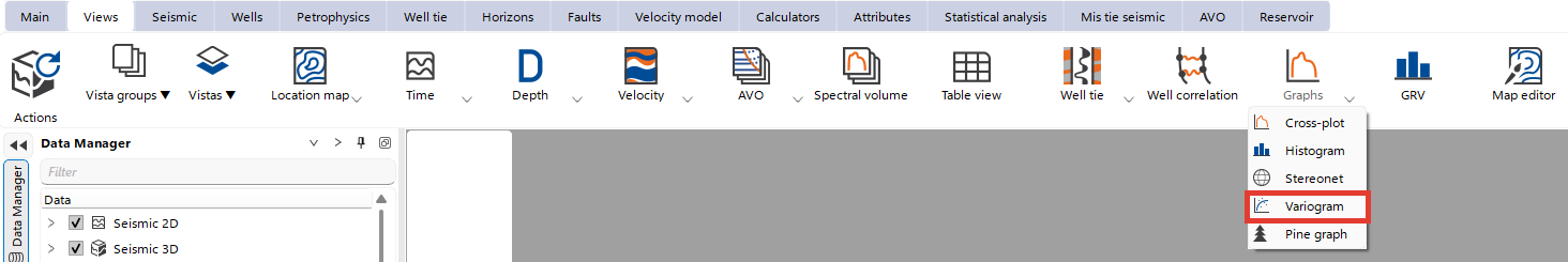
To create Variogram view go to the Views bar, navigate to Graphs and click on Variogram button:
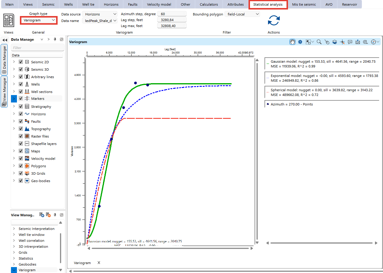
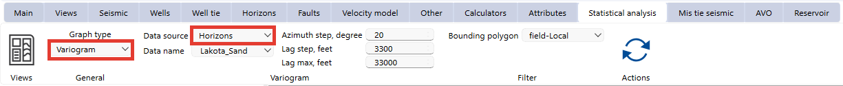
To start variogram analysis, navigate to to the Statistical Analysis bar and select the Variogram option under the Graph type dropdown menu.
Data Sources for Variogram Analysis
1. Well Attributes
Select "Well Attributes" as the data source from the dropdown menu.
Choose the attribute (X, Y, Total depth, KB or Ground level) from the Data Name field.
Specify parameters:
•Azimuth step
•Lag step
•Maximum lag distance

2.Well Logs
Choose "Well Logs" as the data source.
Select a specific well log Data Name field.
Specify parameters:
•Azimuth step
•Lag step
•Maximum lag distance
Additional settings include:
•Value extraction method (Average, RMS, Dominant, Min, Max, Median)
•Range for analysis - between depths or horizons
•Bounding polygon for spatial filtering.

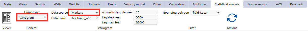
3. Markers
Select "Markers" as the data source.
Choose a geological marker from the Data Name dropdown menu.
Define azimuth step, lag step, and maximum lag distance for spatial analysis.
Additional settings include:
•Bounding polygon for spatial filtering.
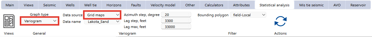
4. Grid maps
Select "Grid maps" as the data source.
Choose a map from the Data Name dropdown menu.
Define azimuth step, lag step, and maximum lag distance for spatial analysis.
Additional settings include:
•Bounding polygon for spatial filtering.
5. Horizons
Select " Horizons" as the data source.
Choose a horizon from the Data Name dropdown menu.
Define azimuth step, lag step, and maximum lag distance for spatial analysis.
Additional settings include:
•Bounding polygon for spatial filtering.
Once you generate a variogram, it appears in the Variogram view. The plot displays experimental variograms as points and fitted models as curves.
Fitted Models:
The tool provides three common variogram models:
Spherical
Exponential
Gaussian
Each model is characterized by:
Nugget: Represents measurement error or micro-scale variation.
Sill: The total variance where the model flattens out.
Range: The distance at which spatial correlation diminishes.
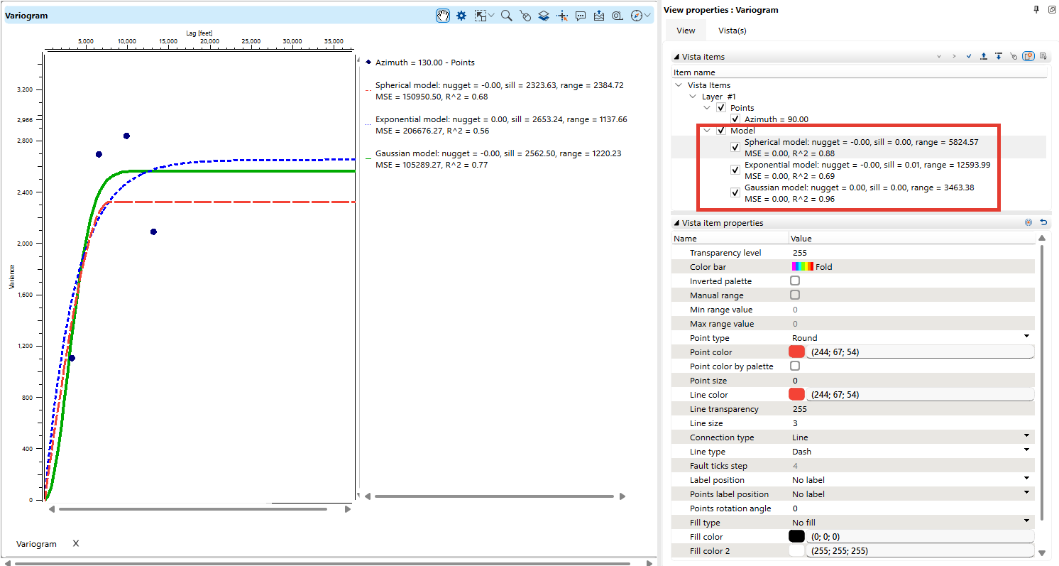
In the Visual Settings panel, users can adjust visual settings for better interpretation:
•Transparency levels
•Color schemes
•Line types and thickness
•Point size and shape
Users can also enable or disable specific models to focus on relevant data trends.