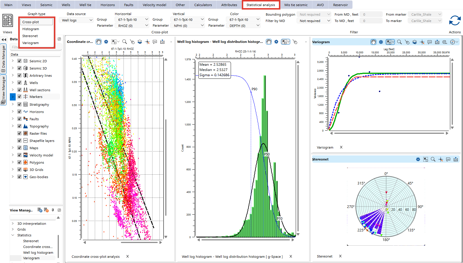
The Statistical Analysis view provides a robust toolkit for analyzing and visualizing relationships between well log attributes, data distributions, and structural orientations.

By selecting the appropriate Graph Type — Cross-Plot, Histogram, Variogram, or Stereonet — users can gain valuable insights into their data through targeted visualization techniques.

For effective analysis, users can fine-tune graph settings such as data source selection, axis parameters, and filters to focus on specific intervals or attributes of interest. The use of Bounding Polygons, MD ranges, and markers allows for precise control over the data included in the analysis, enabling more accurate and meaningful results.

Visual customization is an essential part of the workflow. Adjusting color schemes, point size, and bin settings helps improve clarity and enhances the interpretability of graphs.

Saving graphs to the Data Manager

A graph can be stored in the project, so that it can be reopened later without setting up its parameters again. Right-click the plot in the Cross plot, Histogram, Stereonet or Variogram view and choose the save command of the current graph type, for example Save Cross-plot to Data Manager.... Type a Name for the new object and confirm. The name must not be already used in the same folder.

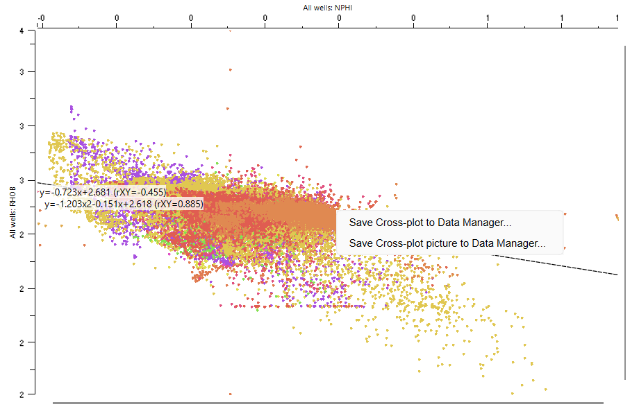
Each of these views also offers a picture command beside the one above, for example Save Cross-plot picture to Data Manager... or Save Histogram picture to Data Manager.... It asks for a Name in the same way and stores a static picture of the graph as it currently looks instead of its settings, in the folder of that graph type next to the saved graphs.

Both commands of a view are also available as buttons in its functional panel, so a graph can be stored without opening the context menu. Point at a button to see which command it runs.

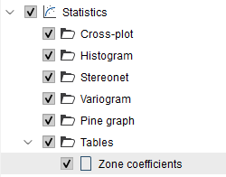
Saved graphs are collected in the Statistics category of the Data manager, which contains a folder for each graph type: Cross-plot, Histogram, Stereonet, Variogram and Pine graph, together with a permanent Tables folder for project tables. The Pine graph folder is filled from the Pine graph view. A saved cross-plot additionally lists the equations of its linear and quadratic regression lines as separate records inside the object.

Right-click a saved item in the Data manager to:

• Open – reopens the saved item. A graph saved from the Statistical analysis view is restored with its graph type, data source, groups, parameters and filters, and that view is brought to the front; a saved picture is shown in a separate window.
• Rename – gives the item another name.
• Delete – removes the item from the project.

A regression record only offers Delete: it keeps the equation of the line as it was when the cross-plot was saved.

Project tables

The Tables folder of the Statistics category keeps tabular data as project objects, for example permeability coefficients per zone, petrophysical cutoffs or core plug measurements. A table is a generic object: it can combine text and numeric columns in any order, it may describe one well, several wells or the whole project, and columns such as a well name, a depth or a zone are used only when the data needs them.

To create a table, right-click the Tables folder and choose New table. Type a Name that is not used by another table in the folder and confirm. The table editor opens on a starter grid of two columns and five empty rows and carries the table name as its title.

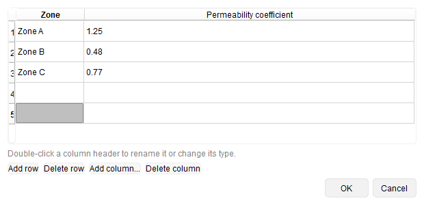
Type the values directly into the cells, and shape the table with the buttons under the grid:

• Add row – adds an empty row at the end of the table.
• Delete row – removes the row of the selected cell.
• Add column... – asks for the Name of a new column and for its Type, Text or Number.
• Delete column – removes the column of the selected cell.

Double-click a column header to rename that column or to change its type. OK stores the table in the project; when a cell of a Number column holds a value that is not a number, the editor names that column and row so that the value can be corrected first.

Data prepared outside the project can be brought in instead: right-click the Tables folder, choose Import table from file and select a Delimited text (*.csv *.txt *.tsv *.dat) file. Answer whether the first row of the file holds the column names, then type a name for the new table; the file name is offered as the default.

Right-click a saved table to Open it in the editor, to Rename it or to Delete it from the project. An open table is written back to the project when the editor is closed with OK.

A table that holds core measurements can also be attached to the well it came from: right-click it and choose Attach to well as core table.... The Attach table to a well as core dialog asks which well the core belongs to, which column is the depth, what the other columns measure and in which units, and stores a copy of the table under that well's Core folder. The project table itself is left unchanged.