To begin with, the statics calculation processes with using tomography algorithm in the g-Platform system based on two main following steps:
1) FIRST BREAK PICKING:
•Module: Refraction FB picking - azimuthal solver guide / phase / aperture;
•Tutorial: First breaks picking.
2) TOMOGRAPHY:
•Modules:
✓Tomo statics 2D/3D.
•Tutorial: Tomography.
Notice that version of the g-Platform used in this tutorial is 5.23811, so all parameters, options, visual QC windows and results may be different from your version.
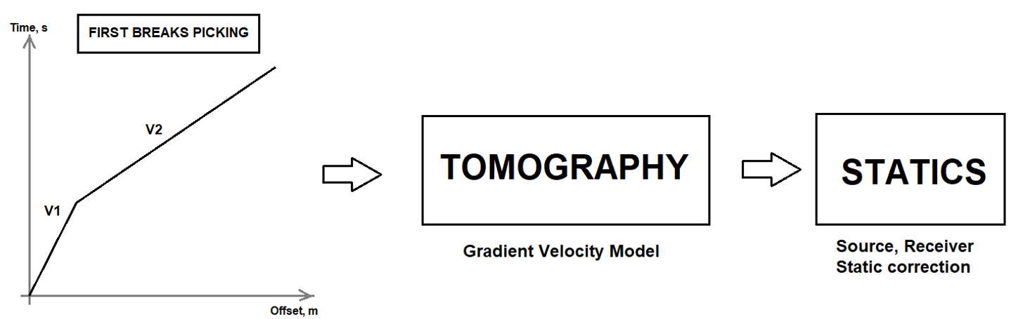
Fig. 1. Scheme of static calculation with using tomography.
Tomography plays a key role in seismic imaging. Be it is a building depth velocity model or calculating the refraction statics by generating the near surface model. Refraction Tomography statics are used in the event of regular refraction statics are not giving optimum results or to improve the refraction statics solution. In this method, the weathering zone (WZ) is parametrized as a number of cells that used for filling up a depth velocity model. Travel times are goes through the cell-model, and residuals times are converted into velocity variations in 2D/3D cells. Here we are able to calculate vertical velocity gradient due to the fact that tomography is a nonlinear move out modeling of the first arrivals (Fig. 2).
The tomographic is sensitive to the initial model due to the fact that the nonlinear solution performs by iterating the ray trace calculation and velocity is updated by local linearization, so the solution of tomography is depending on quality of first breaks picking. Therefore, if we have 2D data set it is more reasonable to make FB picking more accurate by doing it manually.
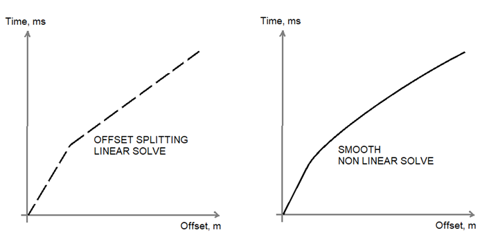
Fig. 2. Linear (left) and nonlinear (right) solutions comparison.
The tomo-statics modules in the g-Platform system are based on the Fresnel seismic travel time tomography. A Fresnel volume approach is applied to represent wave propagation for seismic travel time tomography instead of rays. A Fresnel volume is defined as a set of many waves delayed after the shortest travel time by less than half a period. It is derived by calculating travel times both from a source and from a receiver. Tracing rays from sources to receivers is completely avoided.This considerably reduces computational time. We solved the eikonal equation by using a finite-difference method to calculate travel times. The advantage of this approach is as follows: first, the frequency of wave can be introduced into analysis. Therefore, we can evaluate the resolution of seismic tomography. Next, the smoothing feature can be naturally introduced. Finally, Fresnel volumes with finite bandwidth considerably reduces the sparseness of ray distribution.
The more physically-realistic representation of wave propagation is to treat a ray path as a beam with finite width. Using a Fresnel volume is a natural and an effective approach. A Fresnel volume is a set of many rays delayed after the shortest travel time by less than half the period of wave. The rays in a Fresnel volume are added constructively to form the first-arrival of wave. There have been several studies on the application of Fresnel volumes to seismic tomography since Harlan(1990). In this study, first, we discussed the characteristics of Fresnel volumes. Next, we formulated the inversion procedure. Then, we investigated the resolution of tomography with respect to the frequency (Toshiki W. Seismic travel time tomography using Fresnel volume approach).
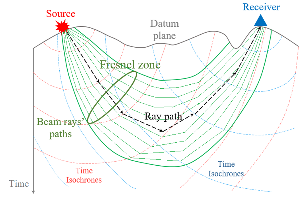
Fig. 3. Travel times scheme.
A module Tomo statics 2D is used for tomography and it requires the first break picks. In this module, it start with an initial model and performs updating the model during each iteration until it converges to the best solution (Fig.4).
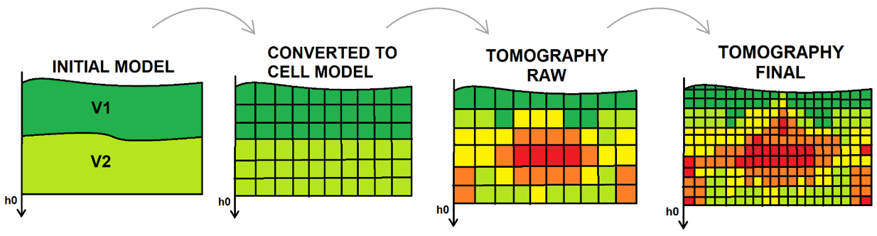
Fig. 4. Scheme of tomography steps.
For the training data in this guide, we use a vibroseis seismic acquisition Poland 2D line that is accessible on the internet free or it is also included to the g-Platform installation (C:\Program Files (x86)\Geomage\gPlatform\demodata\Poland_2D_Vibroseis_LINE_01). Demo data also consists of the FB picking file on your disk in the same folder with the input seismic data set, but you just need to convert ASCII FB pick file into Binary one via Refraction FB picking - azimuthal solver guide / phase / aperture module (import->export). So, we can use the module Tomo statics 2D which requires first breaks as mandatory input data set.
Tomography procedure requires high quality picks, consequently preferable to have manual picking on the 2D line due to relatively small amount of source gathers. The seismic is vibro data and it is another obstacle of using auto picking method as well as trying to use tomography procedure, the result may be far from being sufficiently addressed in comparison with the conventional reciprocal method static solution. Let’s create a workflow which will be consist of all necessary modules for tomography static calculations:
•Read seismic traces: loading seismic data for picking;
•Tomo statics 2D – tomography and statics calculations;
•Static QC – quality control for statics.
For tomography procedure we will use Tomo statics 2D module, add it to the workflow RMB->Modules Next->Find module->Tomo statics 2D and set all the parameters. Notice that the training input data set is located in the g-Platform internal data base (DB), so you need to be sure that geometry assignment step was done properly and all necessary trace headers are updated.
Connect all input data vectors from the previous module of DB:
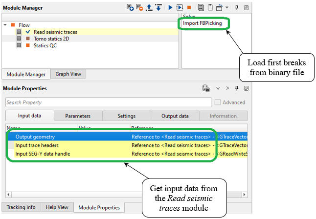
Fig. 5. Tomo statics 2D input parameters.
Usually, testing parameters starts with wider cells size of the model because initially the main goal is to find the most appropriate values for other parameters. When we have optimal result, it is reasonable to reduce cell size and increase the number of iterations. Eventually, a dense gradient depth velocity model is calculated as well as static corrections (ms) for sources and receivers. A depth velocity model may be used for the depth migration step as the upper part of the PSDM model.
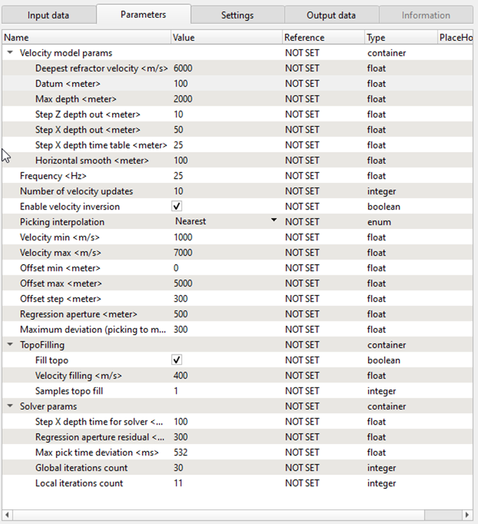
Fig. 6. Tomography parameters.
Tomography parameter explanation:
Velocity model params:
Definition cell-velocity model.
Deepest refractor velocity - the maximum values of guide-wave.
Datum – start value for tomography calculation, constant datum.
Max depth – maximum depth in meters of the model.
Step Z depth out – vertical cell size in meters.
Step X depth out – horizontal cell size in meters.
Step depth time table – vertical step for travel time solution, smaller value – more detailed result, but time consuming.
Horizontal smooth – horizontal velocity smoothing in meters.
Frequency:
Parameter for making solution more detailed in terms of travel time decomposition, bigger value – more detailed result (high spatial frequency), but time consuming. Pay attention on figure 3 Travel times scheme, green constrain depend on this parameter, less frequency - smoothie result.
Number of velocity updates
Tomography iterations.
Enable velocity inversion
Allows to have velocity inversion on the model.
Picking interpolation:
Options for interpolation missing first breaks picks:
Nearest – get picks from the nearest traces, use it in case of small gaps in FB picks.
Regression – model picks by using regression method.
Velocity min
Value for making minimum velocity constrain (m/s).
Velocity max
Value for making maximum velocity constrain (m/s).
Offset min
Value for making minimum offset constrain (m).
Offset max
Value for making maximum offset constrain (m).
Offset step
Step for splitting offset by classes (m).
Regression aperture
Value of aperture for regression algorithm (m), bigger value – smoother solution.
Maximum deviation (picking to model)
Maximum variations of observed picks according into the model trend.
TopoFilling:
Visual parameters for displaying velocity model, it is not used for calculations:
Fill topo
Values above the relief elevations for filling.
Velocity filling – define exact value for filling.
Samples topo fill – how many samples to fill.
Solver params
Residual statics solver parameters:
Step X depth time for solver - Vertical step for residual travel time solution, smaller value – more detailed result, but time consuming.
Regression aperture residual - Value of aperture for regression algorithm (m), bigger value – smoother solution.
Max pick time deviation - Maximum picking variations (ms) for residual static solution.
Global iteration count - Number of global iterations for residual static solution.
Local iteration count - Number of local iterations for residual static solution.
For 3D type tomography Tomo statics 2D/3D there is an option for define the low velocity zone by using Window for calculation V0 parameter which determines an average velocity in the interval (datum - window).
Now we have defined all the parametrization and the next step is launching the tomography calculation by double LMB click on the module or pressing Solve action. To visualize the tomography velocity model and convergence, the user should generate the vista items. The module generates many QC windows: the location map, convergence refraction tomo, tomography velocity view and Current source/receiver/bin gather.
For tomography velocity view, the user can define how many number of iteration required in the parameters tab. Once the solution is computed we can QC the statics result by going to the any one of the current source/receiver/bin gather and enable/disable the Current source gather and Current source gather applied options from the View properties of the Current source/receiver/bin gather. Interactive fast QC by applying statics correction on gathers with different sorting: source, receiver and bin.
Check the source gather before and after statics applying. Choose by LMB clicking on any source on the location map:
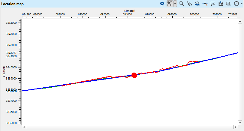
Fig. 7. Source (red) and receiver (blue) interactive map.
And look at the source gather ViewVista window and check gather before and after statics applying:
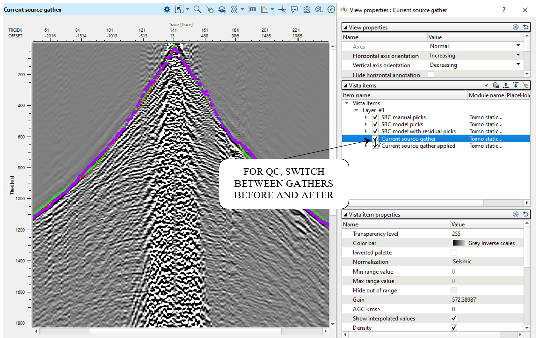
Fig. 8. QC of the resulting statics corrections.
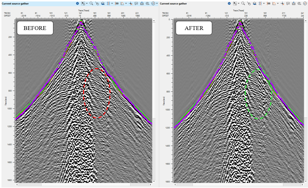
Fig. 9. Source gather before (left) and after (right) tomography statics applying.
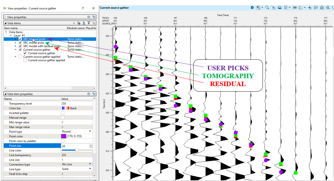
Fig. 10. Source gather and different types of picks for QC: User picks (purple), tomography (green) and residual (red).
Another important QC tool is convergence graphs where you can understand how many tomography iterations should be enough. Every iteration must reduce an error/mistie between observed and modeled times. If the error is too high or the tomo convergence is not matching with the residual convergence then the user can adjust the solver parameters and/or other parameters and click on the Solve option from the action item menu. It will recalculate the solution and update the displays.
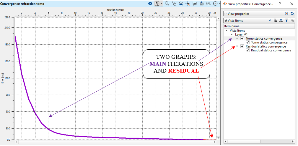
Fig. 11. Graphs of the main-tomography iteration (purple) and residual (red) solution.
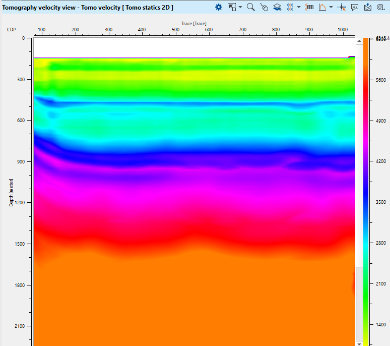
Fig. 12. Depth velocity model after tomography.
The next step is checking statics corrections by using Statics QC module. There are many QC tools like source, receiver statics graphs and maps, source and receiver gathers before and after static applying, tables with static corrections etc.:
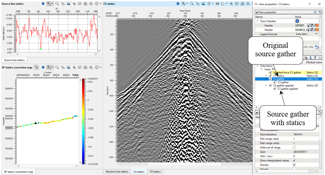
Fig. 13. Statics QC vista windows: source statics graph (left top), source statics map (bottom), source gathers overlaying before and after static correction applying (right).
Finally, we need to apply statics corrections to seismic traces and build a stack section via Stack imaging module that provides wide amount of tools like velocity analysis, stacking, statics applying, etc.
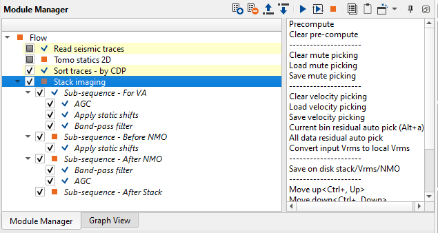
Fig. 14 Workflow - stack creation.
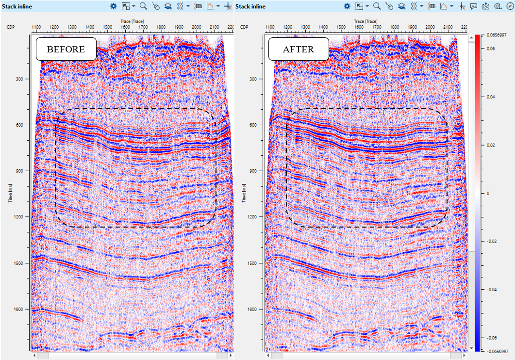
Fig. 15. Stack section before (left) and after (right) tomography statics applying.
* * * If you have any questions, please send an e-mail to: support@geomage.com * * *
![]()
![]()
Toshiki W. Seismic travel time tomography using Fresnel volume approach, 1999 SEG Technical Program Expanded Abstracts.
Cerveny, V. and Soares, J. E. P., 1992, Fresnel volume ray tracing, Geophysics.
Harlan, W. S., 1990, Tomographic estimation of shear velocities from shallow cross-well seismic data.
Luo, Y. and Schuster, G., 1991, Wave-equation travel time inversion, Geophysics.
Matsuoka,T. and Ezaka, T., 1992,Ray-tracing using reciprocity, Geophysics.