2D seismic data can be visualized in g-Space both on a section or within a 3D window, depending on the interpretation needs. Let’s explore how seismic data is displayed in section and review visual settings that aid in picking geological horizons, faults, and other subsurface structures.
In this example, a workspace is prepared in View Manager to visualize 2D seismic profiles. The workspace consists of a Location Map window on the left and a 2D Time Section window on the right. These windows are synchronized for seamless interpretation. The active profile is highlighted in green, and you can easily switch between different seismic profiles, which are visualized both on the map and as seismic sections.
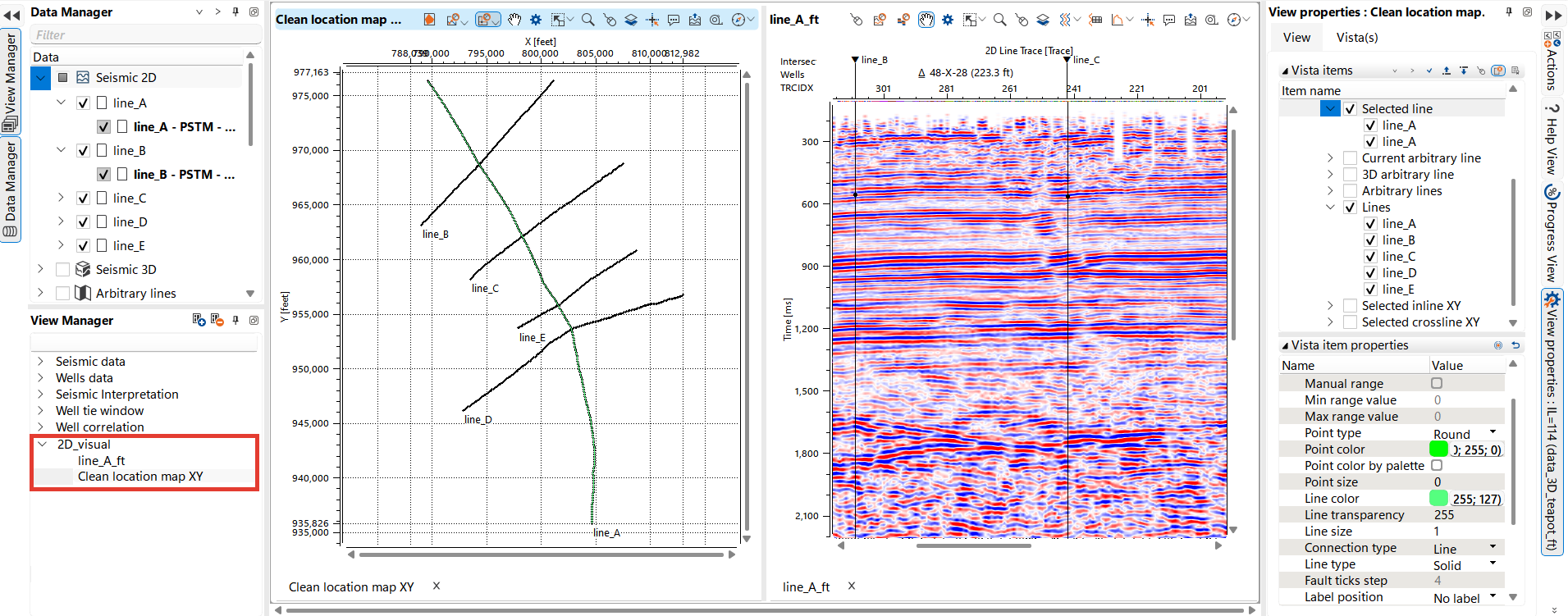
Users can control the appearance of the seismic lines and points by adjusting their properties in the Visual Settings panel. Below is an example of a visual setup of a seismic section.
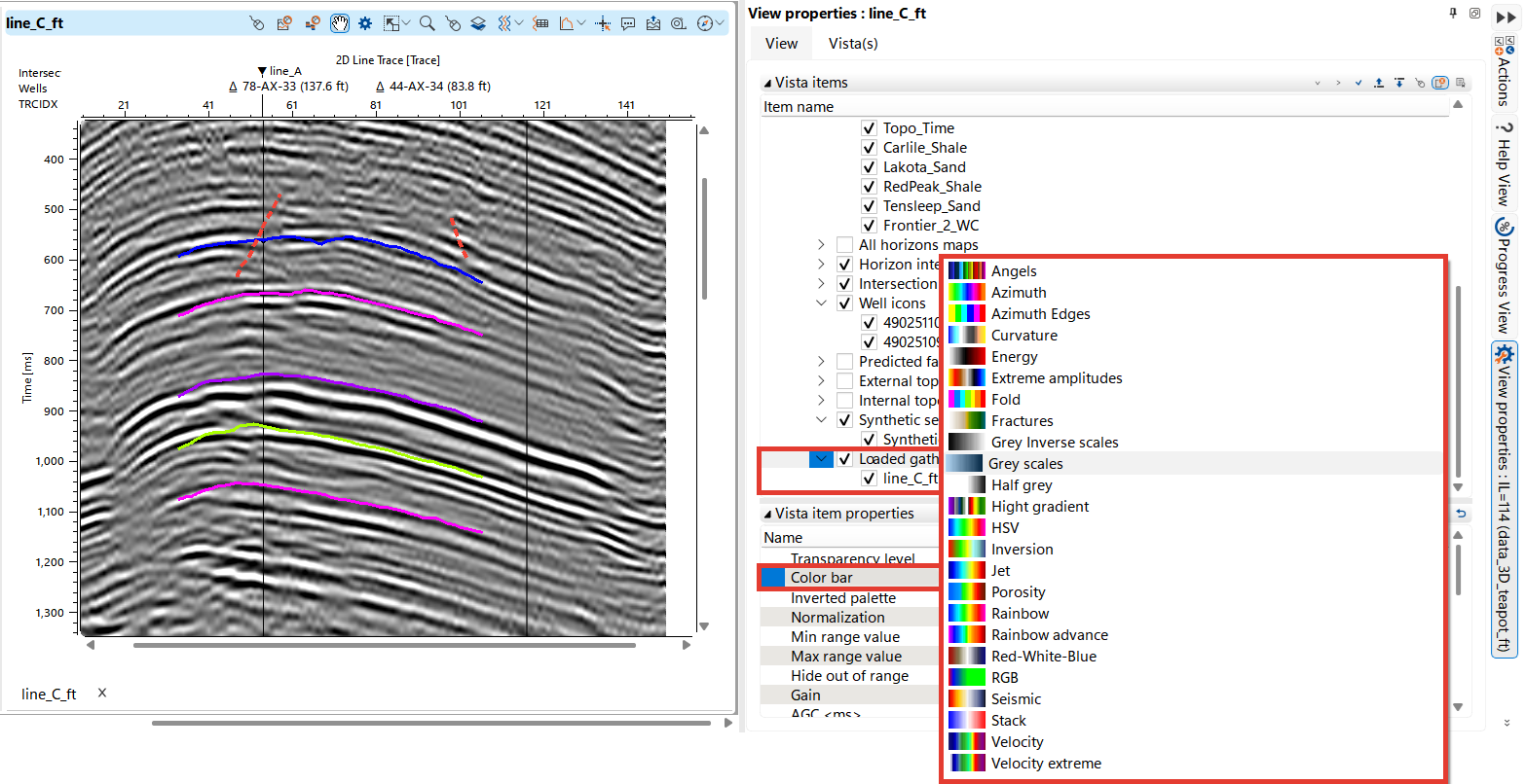
Click on ![]() and the Panel Visual Settings will be opened.
and the Panel Visual Settings will be opened.
There is a list of data that can be visualized in the View. Here, we have shown 3D horizons and fault interpretations on 2D data. You can set a familiar color palette for seismic visualization by clicking on the seismic data, and the settings will be available below in Object Item Properties.
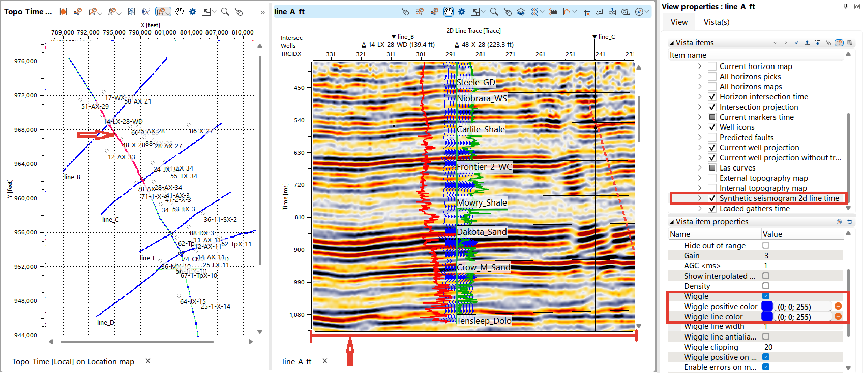
The example of well data visualization on a seismic section in the image below shows the well trajectory, log, synthetic trace, and markers. You can adjust the fill and line colors, the thickness of the synthetic trace, choose to display it as wiggles or in color, and modify the amplitude for the most effective visualization.
The part of the 2D line displayed in the seismic section is highlighted in red on the Map View.
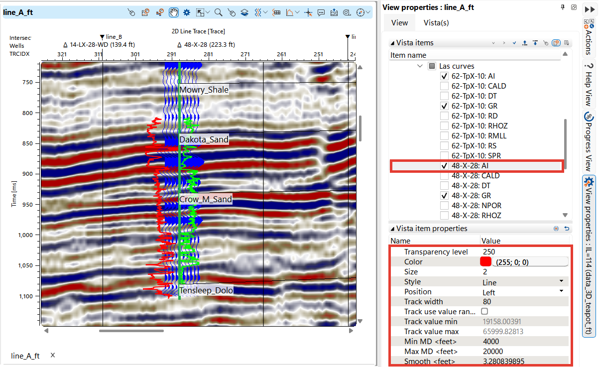
The user has the option to display all logging curves or select specific ones. Settings can be adjusted for all curves by clicking on Las Curves, or for individual curves by clicking directly on the curve name.
In this image, the Acoustic Impedance and Gamma Ray curves have been customized with selected color and thickness, are displayed to the left and right of the well trajectory, and have their tracks width and depth interval modified. Additionally, transparency settings and minimum and maximum value adjustments are available.
Using the Arbitrary Line Tool in g-Space
Arbitrary Line is particularly useful in the following scenarios:
•Comparing 2D and 3D Data: This tool is essential for comparing and assessing the quality of different seismic surveys. By creating custom lines that traverse both 2D profiles and the 3D seismic volume, users can directly compare the resolution and continuity of seismic reflections, leading to a better understanding of the subsurface.
•Correlating Wells: The arbitrary line is helpful for correlating wells, especially when you need to understand the structural and lithofacies features of the interwell space. By drawing a line that connects multiple wells, you can visualize how stratigraphic horizons and structural features change between wells. A detailed description is available in the 3D Data chapter, as these tasks are most commonly handled with 3D data.
•Tying Directional Wells: When dealing with directional or deviated wells, the arbitrary line allows you to create cross-sections that follow the wellbore trajectory. This aids in accurately tying the well data to seismic data, ensuring a more precise integration of well and seismic interpretations.
•Analyzing Geological Structure: For fields with complex geological features, such as the anticline fold in the Demo project, the arbitrary line tool is particularly useful for analyzing geological structures both along and across the fold axis. Given that the fold has a curved structure relative to the geometry of the seismic survey, arbitrary lines enable a more flexible and accurate examination of the fold’s features, which might not align with standard seismic lines.
Notes
Use the Arbitrary Line tool to investigate complex geological structures that might not be apparent on standard inline or crossline sections.
To create an Arbitrary line from 2D profile segments, follow these instructions:
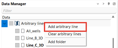
In Data manager click on Arbitrary lines folder and choose Add arbitrary line, a pop-up will open, name the line
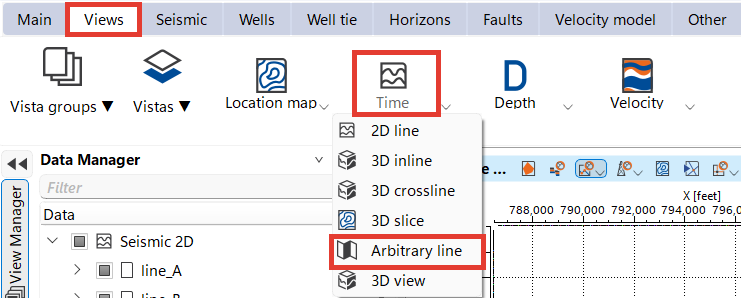
In the View bar select Time, then Arbitrary line. Now there are two Views in Workspace - Location Map and empty Arbitrary line view.
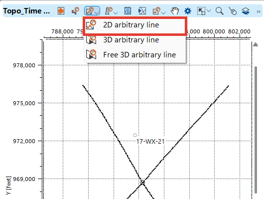
On Map View click Arbitrtary line and choose 2D arbitrary line.
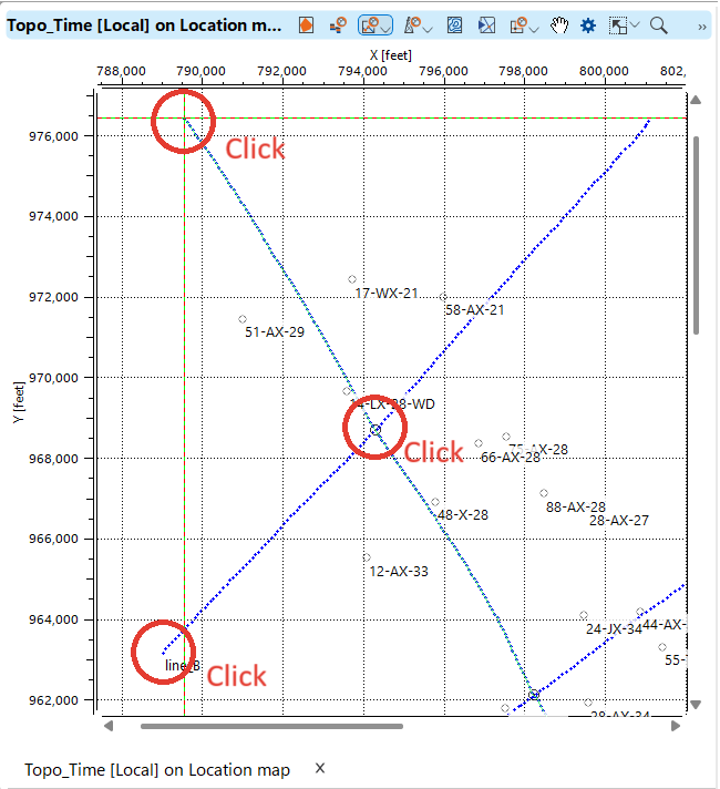
The cursor will change to an active cross. By clicking on the desired 2D line segments, the user will create the geometry of the arbitrary line.
To complete the curve creation, double-click the left mouse button at the last point.
To remove a point from a created arbitrary line, select it by holding down the right mouse button.
A new arbitrary line will be created, you will see it both on the Map and in the Arbitrary line window, the visualization settings can be set in the Visual Settings, in the case below the name of the line is added as well as a color is set.
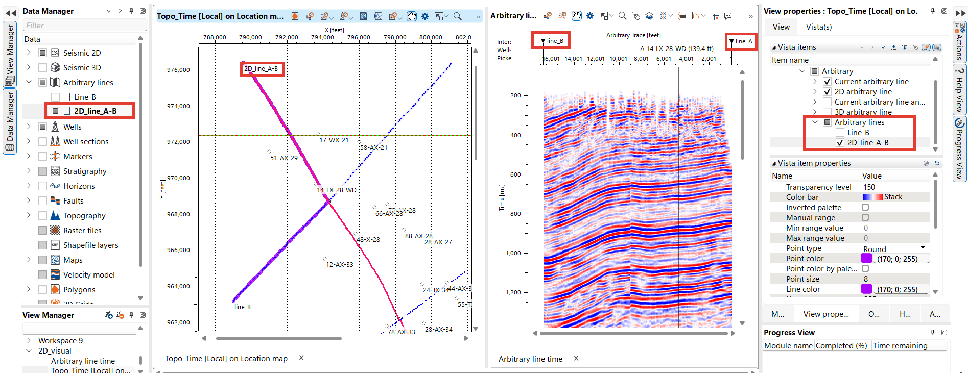
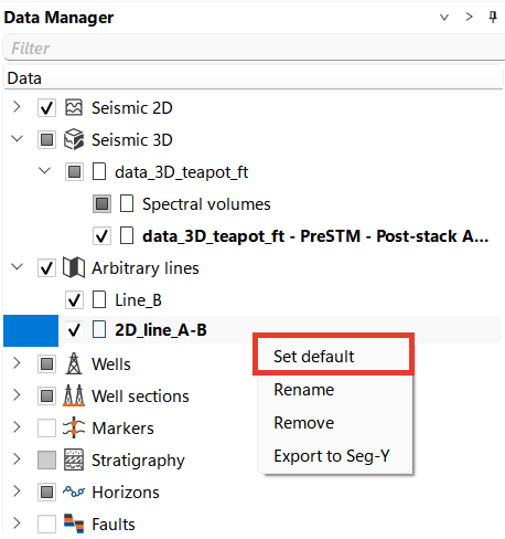
For comparing 2D and 3D Data, make the 2D Arbitrary line (or profile) active in the Data Manager.
Create 2 Arbitrary lines, go to Views - Time/Depth scales, then choose Arbitrary line.
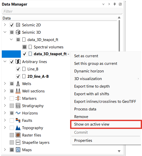
Next, right-click on the 3D dataset you want to visualize and select Show on Active View from the drop-down menu.
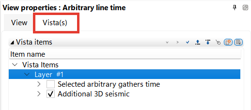
Open the Visual Settings for the Arbitrary line. In the Object(s) tab, select Arbitrary line (2D data at the example below) for one Arbitrary line View and Additional 3D data for the other view, respectively.
A full description of the settings can be found in Seismic View
To synchronize views, go to the Main bar and click SyncViews. Additional settings are available in the drop-down menu.
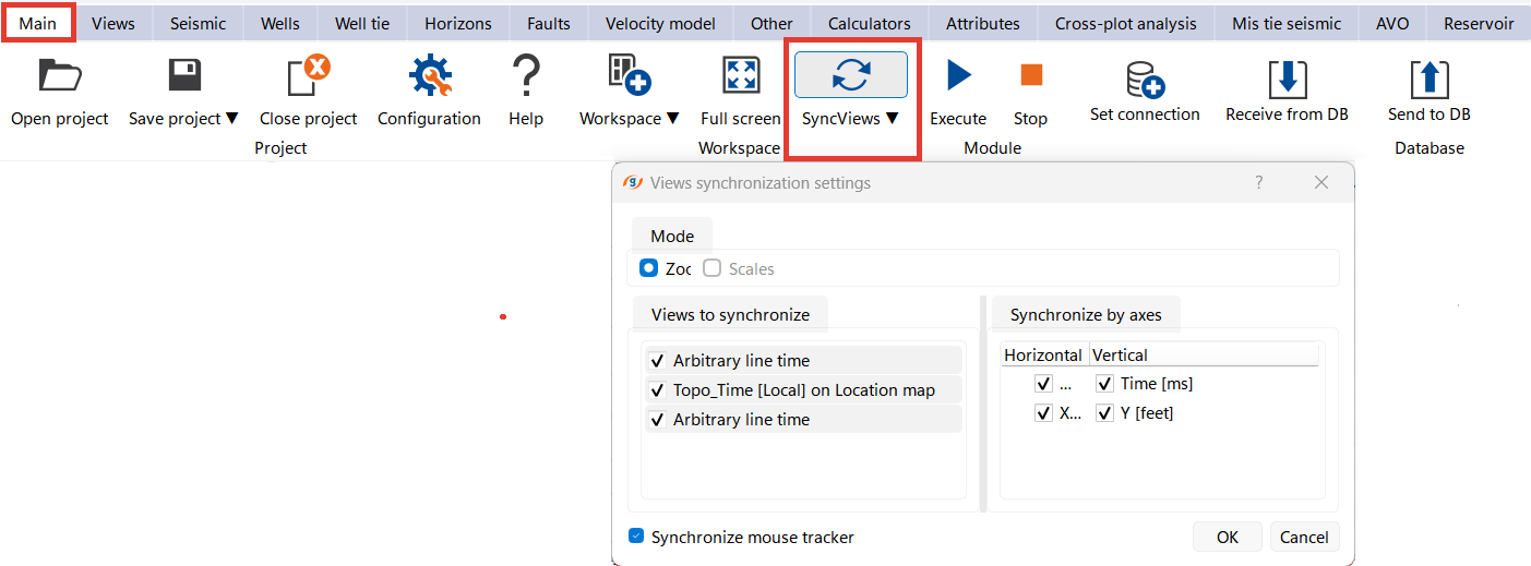
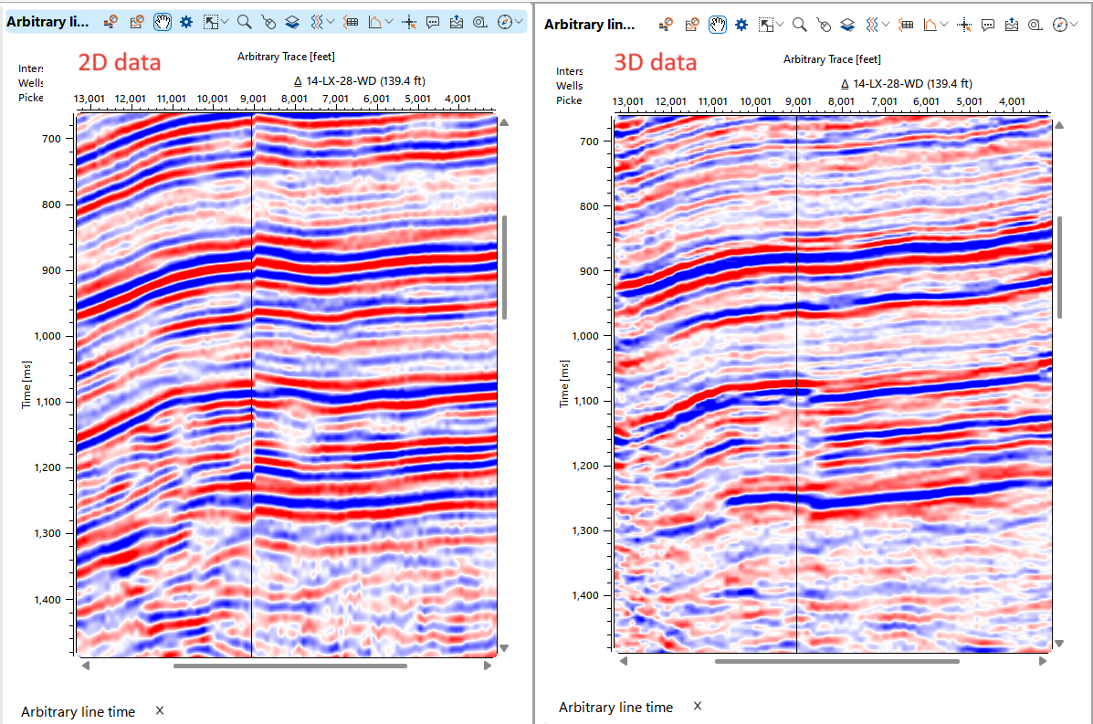
You can now visualize and compare the generated arbitrary lines. In our example, the image below illustrates the comparison results.
This visual comparison helps highlight how arbitrary lines drawn from 2D and 3D data can show differences in the continuity and resolution of seismic events. It’s important to analyze both representations to better understand the subsurface geology.
The 2D data appears smoother with well-defined reflectors, especially in the shallower section. The reflectors are more continuous.
The 3D data in the lower section shows greater variability and more detailed structure, which is common for 3D seismic data, as it provides additional subsurface information.
To display 2D profiles in 3D, select 3D view in time or depth scale depending on your data.
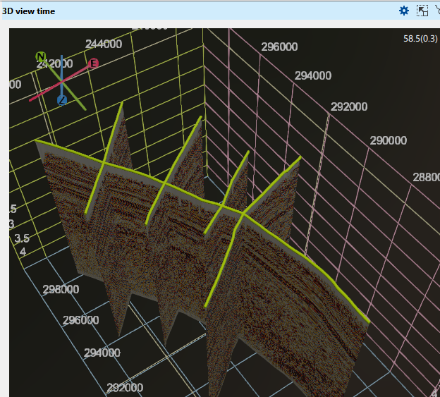
A full description of the settings can be found in 3D View