AVO (Amplitude Variation with Offset) analysis in g-Space allows users to measure rock properties and differentiate between various subsurface materials based on how seismic amplitude changes with offset. Through this analysis, users can generate key parameters like the Intercept, Gradient, and their products to assess the subsurface.
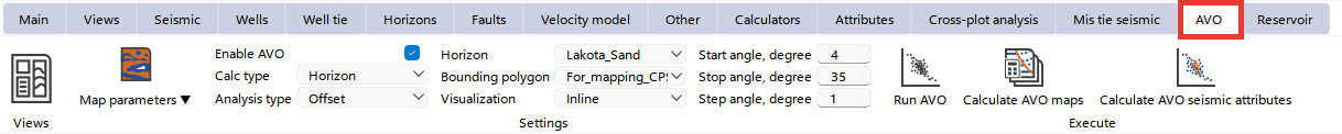
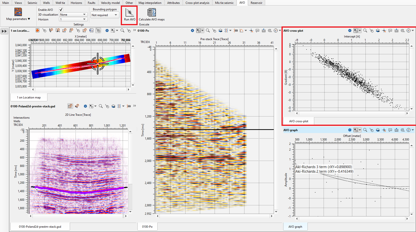
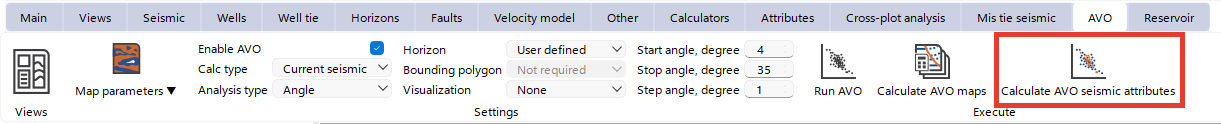
In the AVO tab, there are three main sections:
1.Map Parameters: Where the user can select different AVO attributes like Intercept, Gradient, or their products.
2.Settings: Options to enable or disable AVO, choose 2D/3D visualization, and select available horizons.
3.Execute: The section where the user runs the AVO calculations.
A full description of the functionality is available in the AVO bar
To visualize the output(s) of AVO, the user can open Views in the AVO bar or AVO views in the Views bar.
AVO Analysis procedure
To conduct AVO analysis, you will need:
•Migrated gathers
•Interpreted horizons
Follow these steps for AVO analysis:
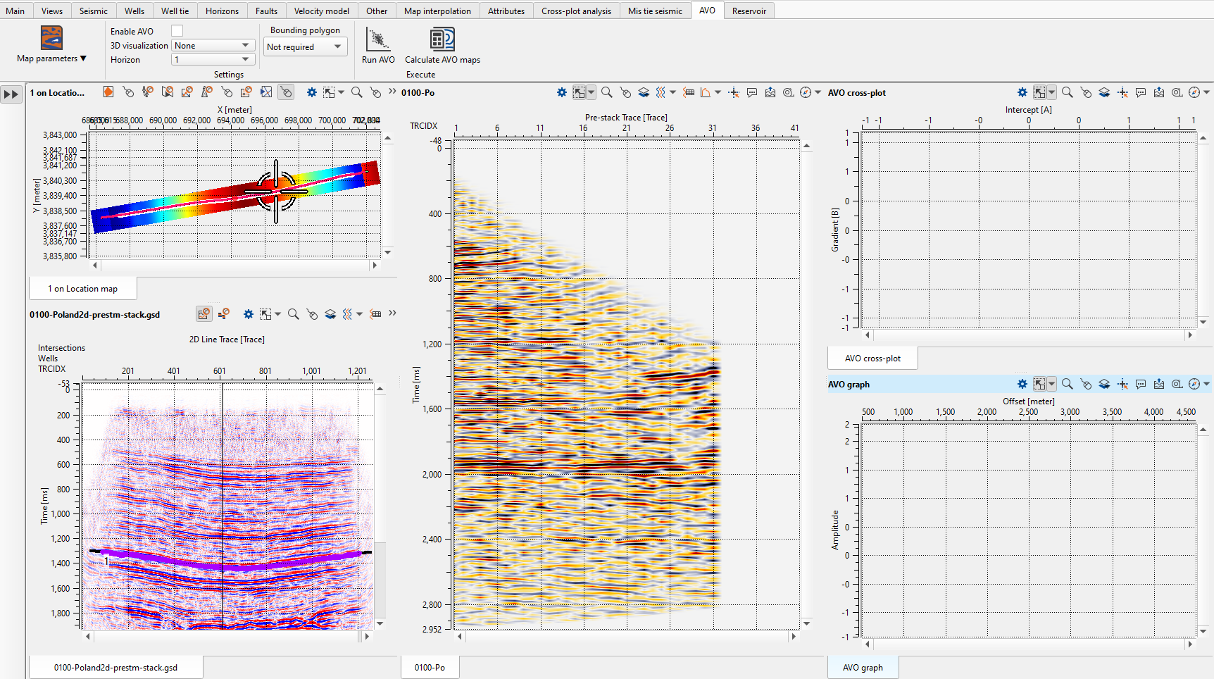
1.Open a New Workspace: Start a new session and add a location map from the Views tab.
2.Select the Image Gather: In the location map, click the Selected image bin icon to display the image bin.
3.Display Object Items: Go to Views and select the appropriate Object items such as Image gather, AVO cross-plot, and AVO graph.
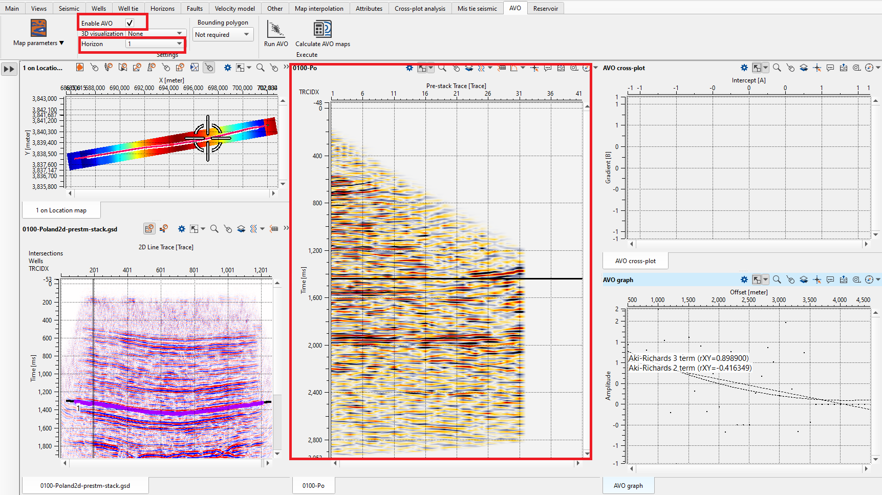
When the Enable AVO option is selected, the current horizon (displayed as a black line on the image gather) will appear along with the AVO graph. The user can then run AVO calculations, which are displayed on the AVO cross-plot.
Now click on Enable AVO option. It will display the Current Horizon (black line on the image gather) along with AVO graph with Aki-Richardson regression graphs as shown below.
To generate the AVO cross-plot, click on the Run AVO icon. It will create the cross plot as shown below.
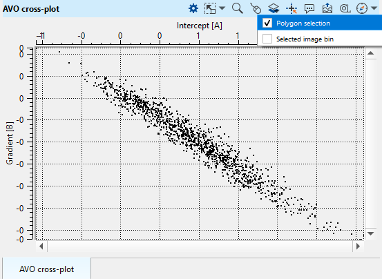
Inside the AVO cross-plot view, the user can pick a polygon and the corresponding bins falling inside the polygon are display on the location map. To pick a polygon, select Control item icon on the AVO Cross-plot view.
It will pop-up a window. Give a name to the polygon.
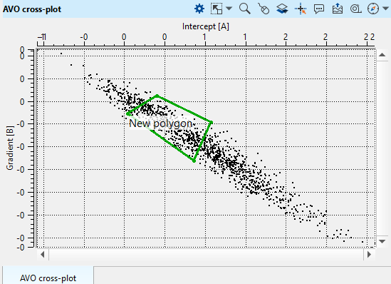
Picking a Polygon on the Cross-Plot
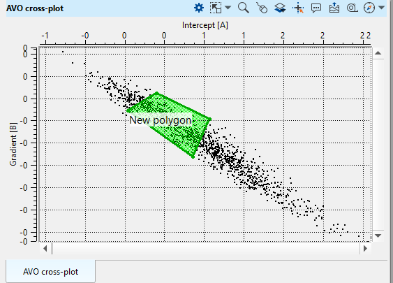
Once the AVO cross-plot is generated, users can pick polygons to analyze specific data points. Clicking on the cross-plot display allows for polygon picking, and these polygons will correspond to bins on the location map. Users can also assign different colors to polygons for better visual analysis.
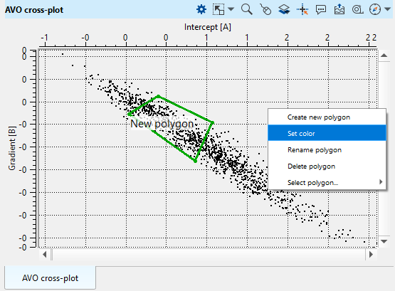
Now hold ALT+Right click to get more options. Here the user can choose different options like create a new polygon or set a color to the existing polygon etc. We selected Set color option as shown below.
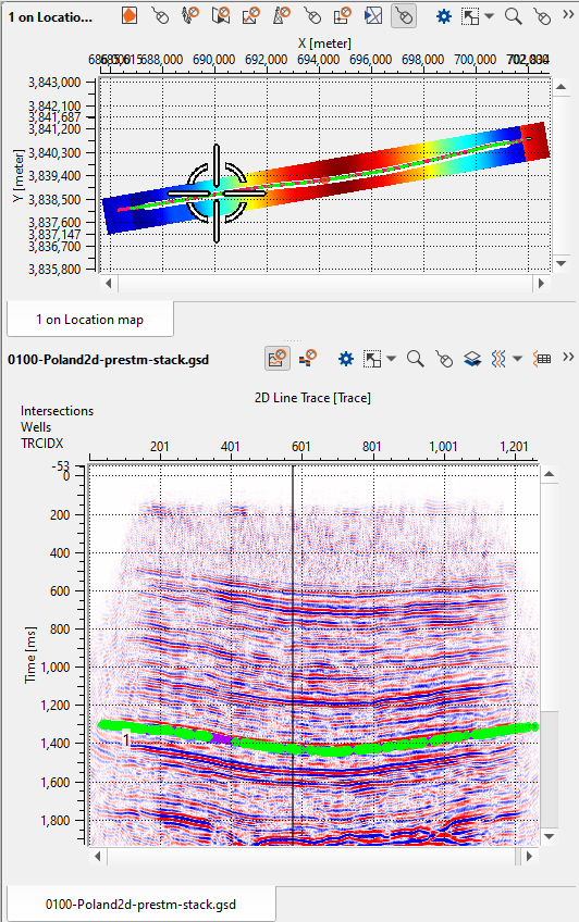
Within the polygon, whatever the bin points present will be displayed on the location map as well as on the picked horizon. All the green dots on the location map are the corresponding bins within the polygon.
Calculating AVO Maps
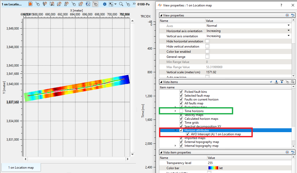
To calculate AVO maps, such as Intercept and Gradient, the user should select the appropriate options from the Map Parameters drop-down menu and click Calculate AVO Maps. The outputs will be available under the Visual Settings of the location map, where the results will be stored under the Horizon Attributes.
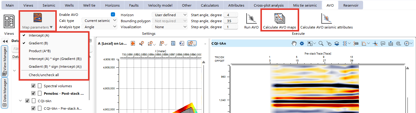
In the example below, there is the Intercept option is selected. The output of the Intercept should be available at the Visual Settings of the Location map under Horizon Attributes
Note
| To view the attributes, first uncheck the Time horizons Object items |
In the Calculating AVO seismic attributes section, users can configure and compute various AVO parameters such as Intercept, Gradient, and other derived attributes. Click on Calculate AVO seismic attributes in the AVO bar
The Calculate seismic attributes wizard will be opened
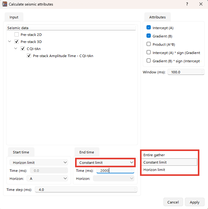
In the Seismic data panel, select the dataset for AVO analysis. Available data types may include Pre-stack 2D and Pre-stack 3D.
Then set the Start time and End time intervals for the AVO calculation:
Start time: Choose either a specific time in milliseconds or set a Horizon limit or the Entire gather to define the start boundary based on a seismic horizon.
End time: Similarly, you can set the end boundary.
In the Attributes panel, choose which seismic attributes to calculate. Define the time window (in milliseconds) over which the attributes will be calculated.
Once all parameters are configured, click Apply to begin the calculation. The selected AVO attributes will be generated for the defined time interval and data range.
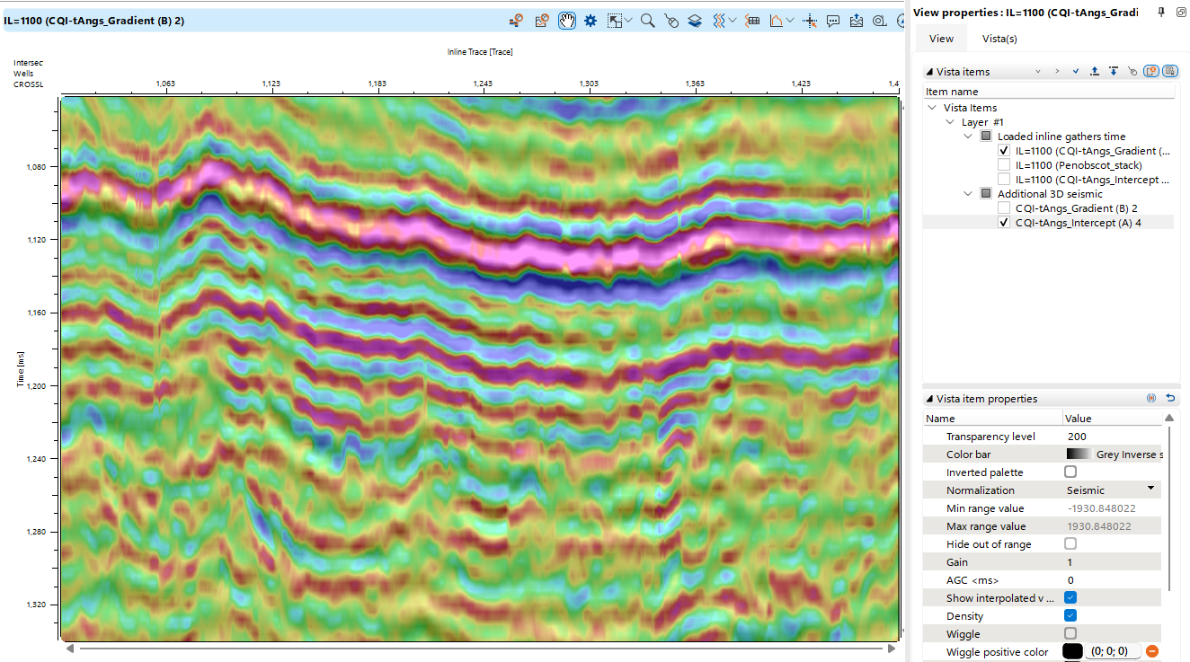
After computation, the results will be stored in the Seismic folder in the Data manager and can be visualized in the AVO views.
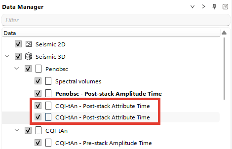
Users can adjust visualization settings such as transparency, color bar, and density options in the property panel to refine the display for more detailed analysis.