Well Tie view in g-Space is a powerful tool that allows you to visualize and analyze well data, generate synthetic seismograms, and perform seismic-to-well tie operations.
Preparing for Well-to-Seismic Tie
To perform a seismic-to-well tie, you must have the following data loaded:
•Seismic Data: 2D lines or 3D volumes.
•Well Information: This includes check shots, sonic logs, density logs, and optionally, impedance data.
Subscribe to our channel and watch the video on how to perform Well tie in g-Space on YouTube
In this chapter, we will guide you through the well-to-seismic tie process using the Demo project for the Teapot oil field.
We will focus on the well 67-1-TpX-10, which is equipped with sonic and density logs, as well as checkshot data. The goal is to tie this well to a 3D seismic volume by generating a synthetic seismogram, comparing it to the seismic composite trace at the well location, and then analyzing the outcomes.
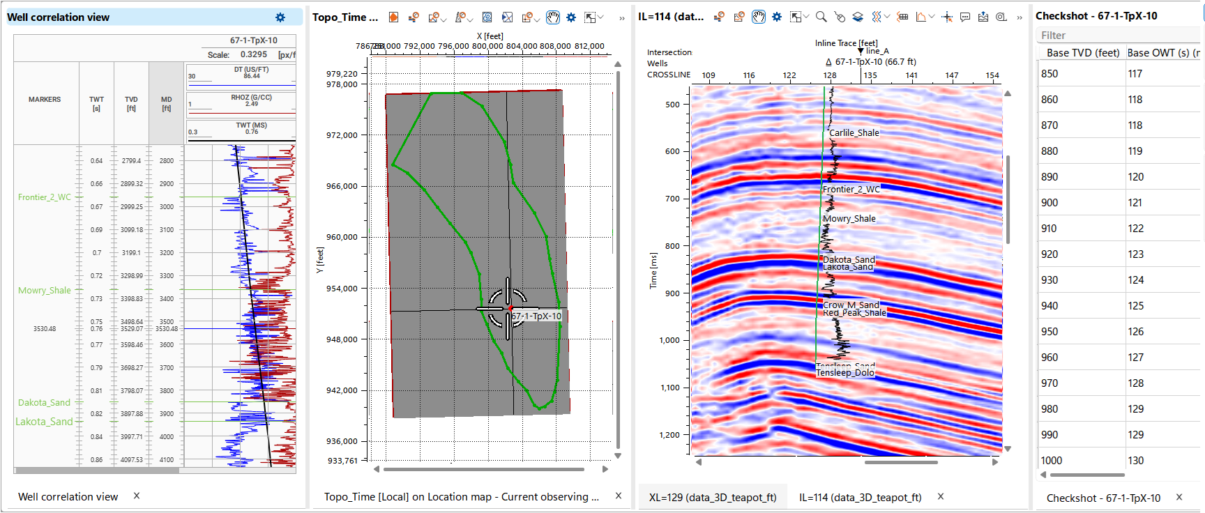
Let's have a look at the data
Well Correlation View (left panel) is used to visualize the well logs, including the sonic and density logs for well 67-1-TpX-10. The logs are plotted against depth and time. Markers are annotated alongside the logs, aiding in the correlation with seismic data.
Location Map displays the position of well 67-1-TpX-10 within the seismic survey area.
Inline Seismic View shows a vertical slice of the 3D seismic volume passing through the well location.
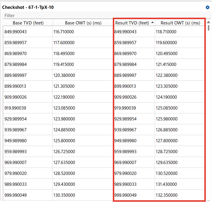
Checkshot Table View (right panel) provides a checkshot data for well 67-1-TpX-10, which includes both True Vertical Depth (TVD) and One-Way Travel Time (OWT). Well correlation view automatically recalculates and displays TWT values along its axis.
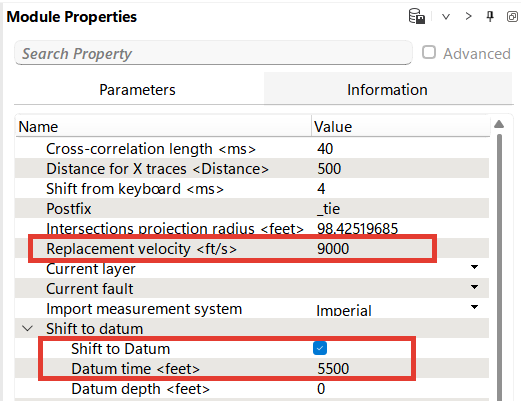
Please verify the 3D seismic reference level and replacement velocity in the Module Properties. Ensure that the Datum is set to 5500 feet and the Replacement Velocity is set to 9000 ft/s.
Navigate to the Well Tie Bar, which will be the workspace for this process.

Setting Up the Well Tie Bar
The Well Tie Bar is divided into three main sections: Seismic, Synthetic, and Cross-correlation.
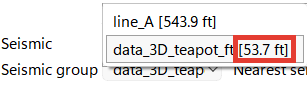
Seismic section (highlighted in red) allows the user to select the seismic lines or volumes that are near the selected well. It displays options to choose specific seismic data from the drop-down menu, such as the seismic volume or group. In this Demo project, we will be performing the well tie to a 3D seismic volume.
The Nearest Seis Distance field displays the distance from the selected well to the nearest seismic line or volume. For example, in this case, the distance is 53.7 feet.
The user can define a specific distance for the nearest seismic data using the Nearest Seis Distance setting. For instance, if a distance of 1,500 feet is specified, only seismic lines within this radius from the well will be considered.
Nearest Seis Width defines the number of seismic traces to be displayed around the well location. In this case, we set it to 50 traces.
Synthetic Section (highlighted in green) is dedicated to generating and analyzing the synthetic seismogram. It includes tools for creating synthetic traces based on the sonic and density logs and performing wavelet analysis.
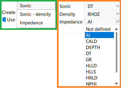
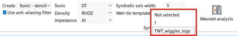
To create the synthetic curve, you need to specify the type of data that will be used in the process. In our scenario, we have both acoustic (sonic) and density logs available. To proceed, in the drop-down menus (highlighted in orange), select the appropriate curves that correspond to the available data:
•For the Sonic log, choose the curve labeled DT
•For the Density log, select the curve labeled RHOZ
Use anti aliasing filter we will set by default, checked.
Synthetic Seis Width allows you to define the width of the synthetic seismogram by specifying the total number of seismic traces to include. For our project, we will set this value to 1 trace to generate a single synthetic trace.
To visualize the well-to-seismic tie process, start by creating a new workspace in the View Manager.
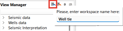
To display the tie, you'll need to include a Location Map where the wells will be displayed. As you choose a well with time-depth data, it will be visualized at Well tie View.
Following this, create a Well Tie View by clicking  from the Well tie bar. This function is also available in Views Bar, choose the same button Well tie.
The default Well Tie View will open in front of you. Let's review and configure it.
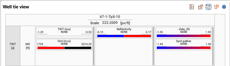
The display consists of three tracks showing the following data:
•Two Way Time
•Interval velocities
•Synthetic trace
•A seismic section with the synthetic trace overlaid at the well intersection
You can also check all the settings in the Module Properties panel.
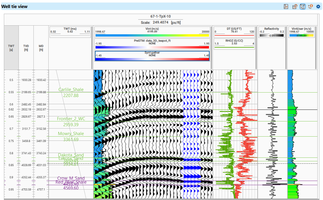
Let's configure the template and adjust it to a view that suits your preferences. The full settings description for Well Tie View are available here. The curve settings are similar to the settings in Well correlation
By right-clicking, you can access global settings, where you can easily add scales, such as TVD, which is especially useful for horizontal wells.
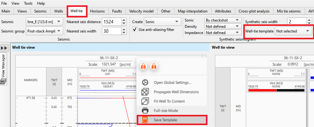
For this example, the seismic section was configured to display as wiggles, and the number of synthetic traces was adjusted for easy visual comparison. Markers were also visualized along with the well logs to enhance the interpretation.
To save the settings as a template, right-click in the well name field and select Save Template.
To apply the template, navigate to the Well Tie Bar and select the desired template from the drop-down menu.
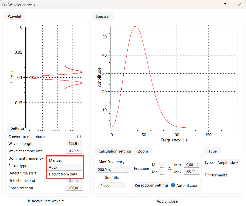
The Wavelet Analysis option allows for the selection or extraction of a wavelet, which is used to generate the synthetic seismogram.
By default, the system uses a Ricker wavelet, but the user has three options for wavelet creation:
1.Manual: The user can design the wavelet by specifying parameters according to their specific requirements.
2.Auto: The wavelet is automatically generated using the input data, but the wavelet type remains Ricker.
3.Detect from Data: The system detects and extracts the wavelet directly from the input seismic data, allowing for a more customized wavelet that matches the actual data characteristics.
Additionally, users can save the synthetic trace to a LAS file for further analysis.
If the user makes any parameter changes in the wavelet analysis window then they should click on Recalculate wavelet and then on Apply and Close to commit the changes to get the updated wavelet and synthetic trace.
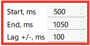
Cross-correlation section handles the cross-correlation process between the synthetic seismogram and the seismic data. It includes settings for the time range (start and end times) and the lag in the Well tie bar. The user can adjust these settings to optimize the match between the synthetic and seismic data.
Note
For accurate results, it is recommended to set the cross-correlation calculation window to at least 2-3 wavelet lengths.
Let's move on to Seismic to Synthetic Comparison and Time-Depth Adjustment
Begin by identifying and matching known reference reflections between the seismic and synthetic data.
Activate the anchor change function. Then, select a reference reflection and double-click the left mouse button to place an anchor on it. Anchors act as tie points, allowing users to align the seismic data with the synthetic trace. Hold the left mouse button to drag and position the anchor at the desired interval.
For optimizing the correlation, use the auto-shift function, which automatically adjusts to achieve the maximum cross-correlation coefficient.
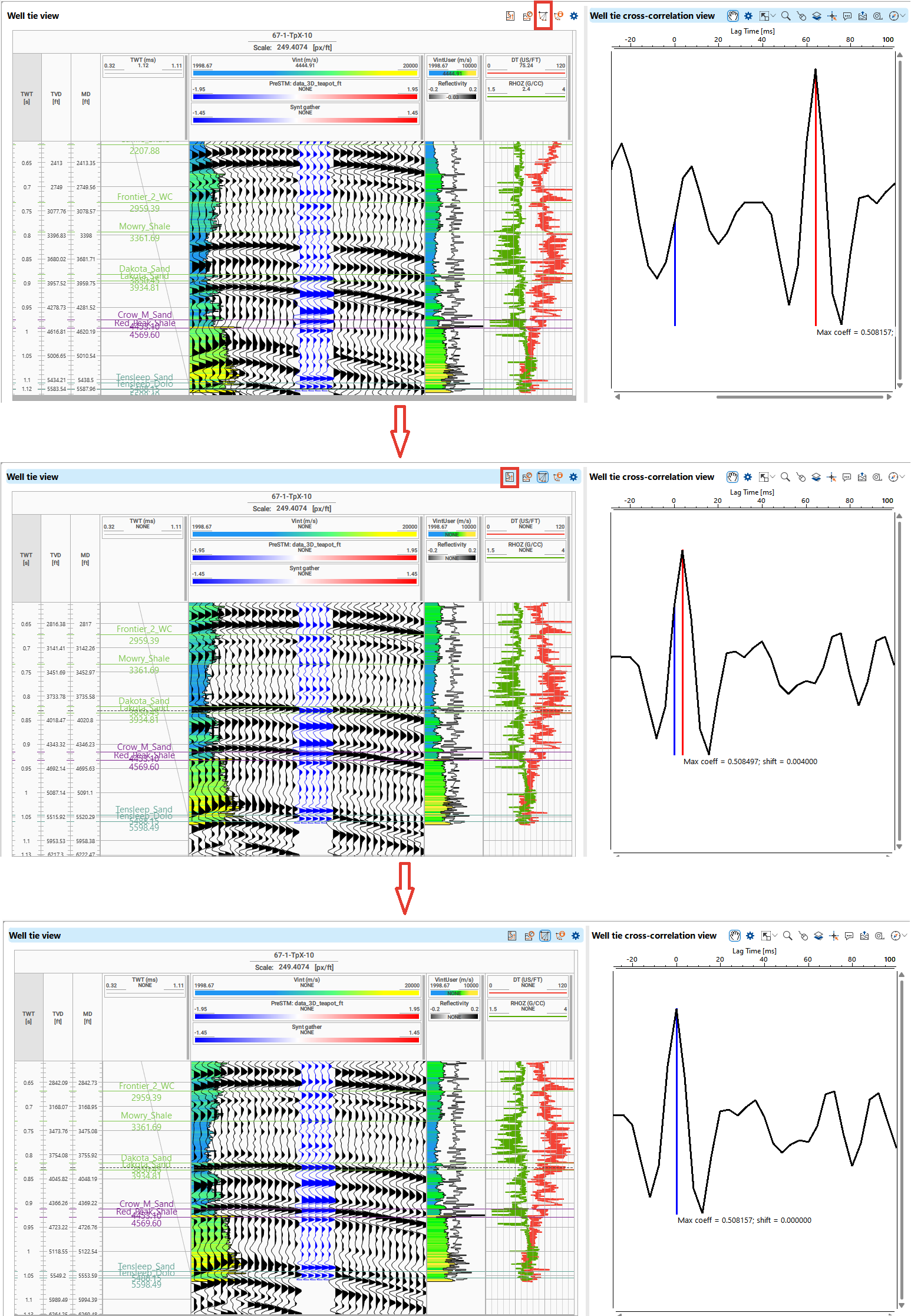
If you are working on a specific interval, we recommend reducing the correlation interval and placing a series of anchors over a larger scale. Visually inspect the alignment of key reflectors between the synthetic and the seismic trace. And correlate them by using anchors (highlighted in red on picture below).
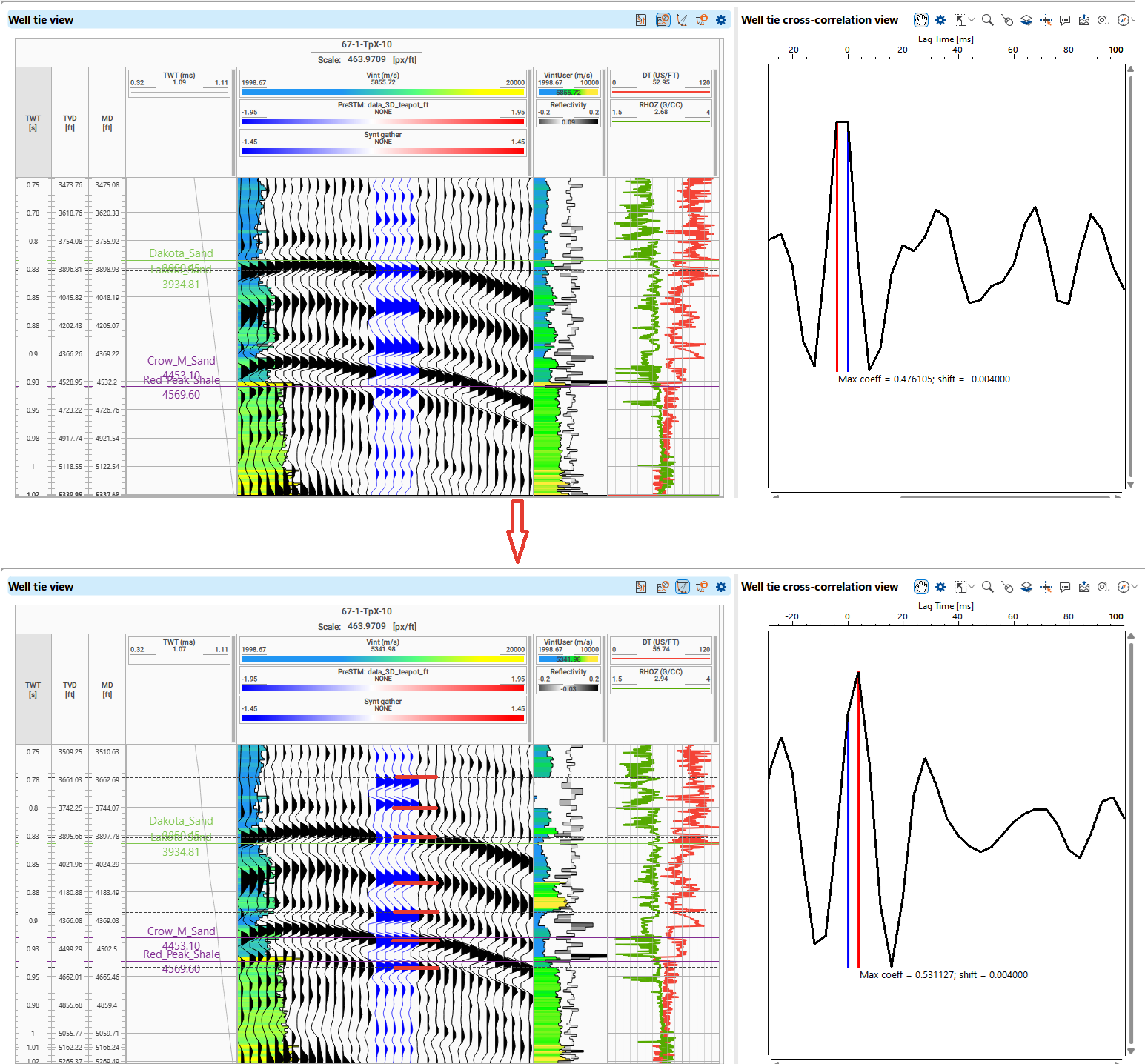
Note that as the curve changes, you see changes in the cross-correlation graph and in the time-depth table. There are two new columns for Result TVD and result OWT.
To delete the current version of your checkshot, select Remove All Anchors from the top menu. This will also update the checkshot curve.
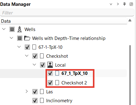
In g-Space, you can upload multiple checkshots. To perform a well tie, select the active checkshot in the Data Manager by double-clicking on it.
Creating a check-shot from sonic log
If the wells with Sonic logs are not loading for well-tie, please perform the following steps:
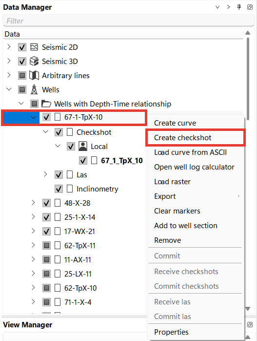
1. Create a new checkshot for this well in the Data Manager; make sure that this checkshot is active.
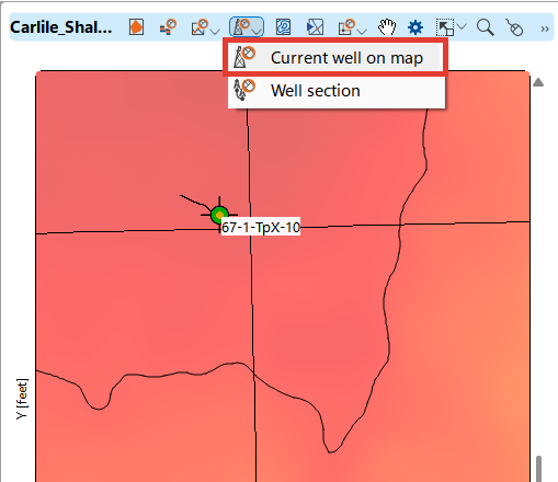
2. Go to Location map and select "Current well on map" icon ![]()
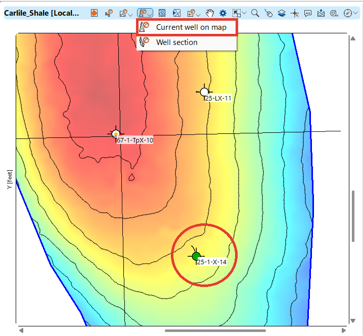
Click on the well and it will display a new window as shown below
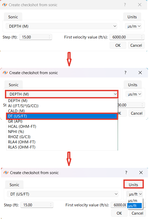
Now set the curve corresponding to the sonic from the drop-down list, in our case DT log, and make sure the units are correct.
Set Step for checkshot and First velocity value
Notes
1.The process of generating a checkshot from a sonic log involves using the sonic log data to estimate the travel time of seismic waves through the subsurface. A sonic log provides interval transit times (Δt), which is the time it takes for a sound wave to travel through a unit length of rock. By integrating these transit times over the depth of the well, we can calculate the cumulative travel time and create a synthetic checkshot.
2.However, the sonic log often does not cover the uppermost part of the well, leaving a gap in the data. In such cases, the user must manually set a velocity value for the first available depth in the log. This user-defined velocity serves as an approximation for the travel times through the upper layers that are not recorded in the sonic log.
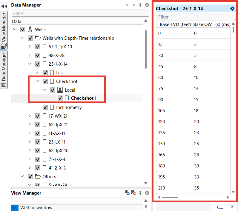
User can see the created checkshot in the well folder in the data manager and open it as a table
Once satisfied with the tie, finalize it by saving the synthetic seismogram and the adjusted Time-Depth curve.
Notes
1.Datum Level Consideration. The datum level represents a reference point, usually the mean sea level or another fixed elevation, from which depths are measured. Ensuring that all wells and seismic data are tied to the same datum level is essential to avoid misalignments.
2.Understanding Different Data Scales and Resolutions. Be aware of potential mismatches in resolution when correlating seismic and well data. For example, subtle geological features visible in well logs may not be as apparent in seismic data.
3.Reviewing Log Data for Errors. Log data may contain errors, such as spikes, shifts, or inconsistent readings, which can lead to incorrect synthetic seismograms and false reflections. A thorough review of the log data by a petrophysicist is recommended before proceeding with the well-to-seismic tie.
4.Calibration with Checkshot Data. Always calibrate your well logs against checkshot data, if available. Checkshots provide more accurate time-depth information and help correct any discrepancies between the log-derived and actual time-depth relationships. Cross-verify the time-depth data with multiple sources, such as VSP (Vertical Seismic Profiling) data, to ensure consistency and accuracy.