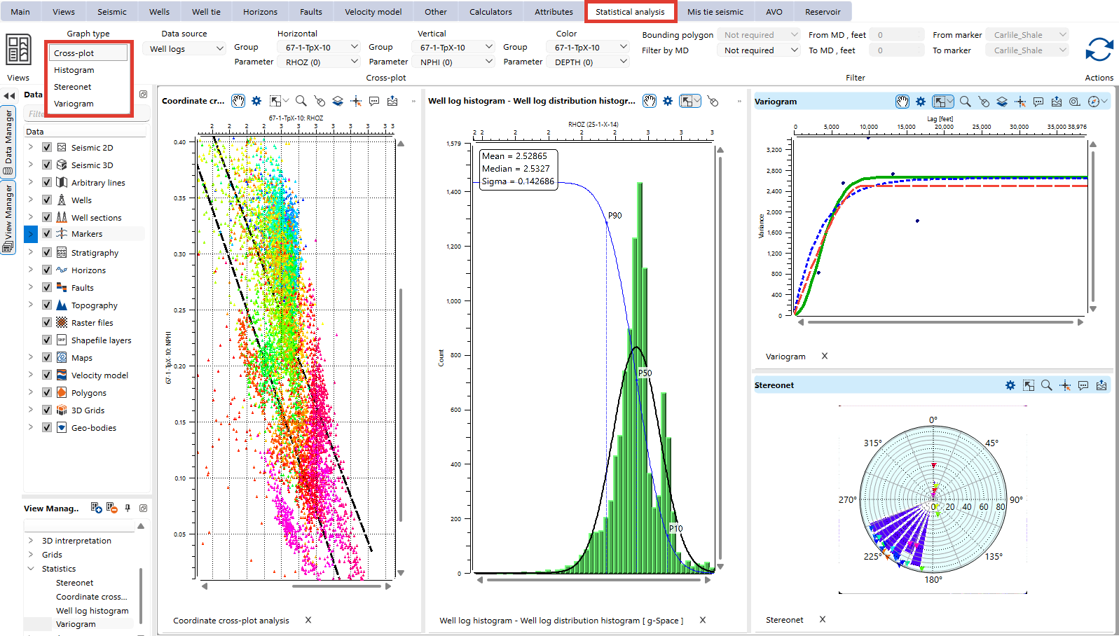
Statistical analysis view in g-Space is a powerful tool for analyzing and visualizing relationships between different attributes.
It provides three graph types:
1.Cross-plot
2.Histogram
3.Variogram
4.Stereonet View
5.Pine graph
Each graph type serves a unique purpose in analyzing subsurface data and identifying trends, patterns, or distributions.
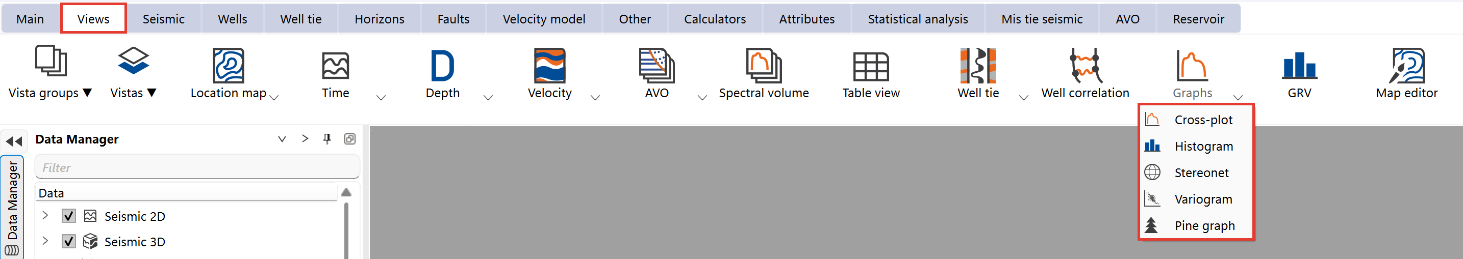
To access these Views:
1.Navigate to the Views Bar in the Ribbon.
2.Select the Graphs option.
3.Open the desired graph type: Cross-plot, Histogram, Variogram, Stereonet or Pine graph View.
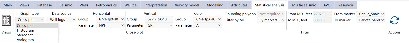
In the Statistical Analysis Bar users can configure their plots.
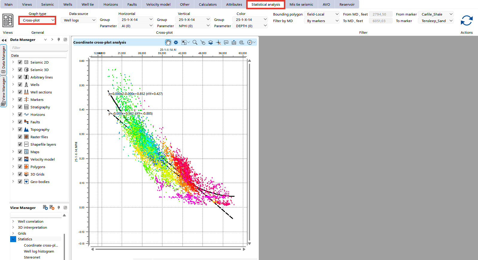
Cross-Plot view is used to visualize the relationship between two selected attributes (X and Y axes). This is particularly useful for identifying correlations or patterns between the two variables.
Data Source: Choose the type of data to analyze (e.g., Well Logs or XY Data).
Horizontal Axis: Select the Group and corresponding Parameter for the X-axis.
Vertical Axis: Select the Group and corresponding Parameter for the Y-axis.
Color: Optionally assign a parameter for point coloring to enhance visualization.
Bounding Polygon: Limit points displayed on the cross-plot using a predefined polygon.
Filter by MD/Markers: For well data, filter points within specific measured depth (MD) ranges or between selected markers.
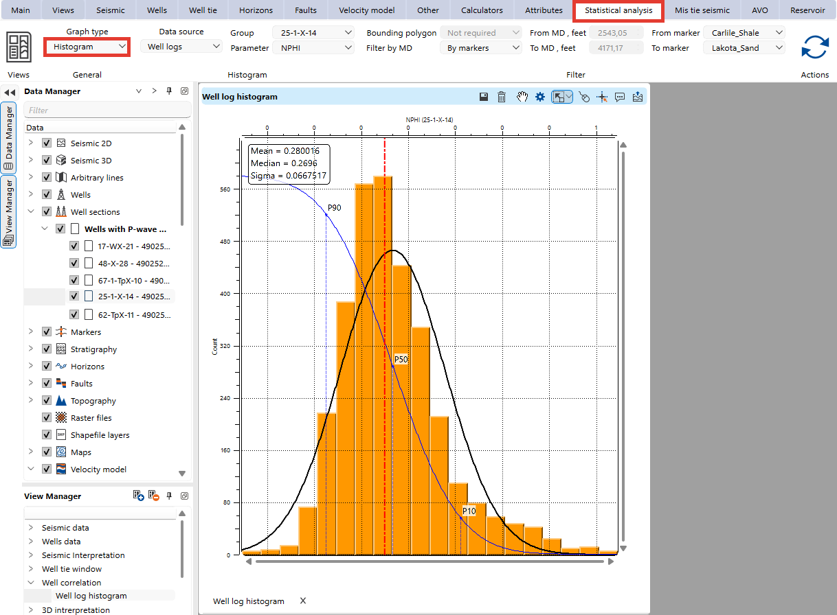
Histogram view provides a graphical representation of the distribution of an attribute, giving users insights into the frequency and range of data values.
Data Source: Choose the type of data to analyze (e.g., Well Logs or XY Data).
Group: Select the well log group to be analyzed.
Parameter: Choose the parameter to visualize.
Bounding Polygon: Limit points displayed on the cross-plot using a predefined polygon.
Filter by MD/Markers: For well data, filter points within specific measured depth (MD) ranges or between selected markers.
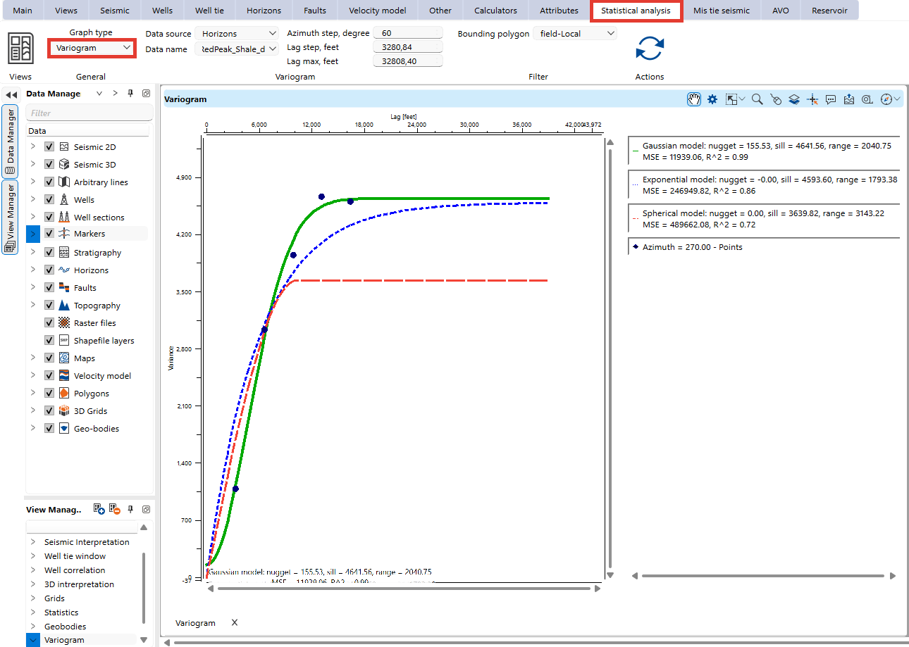
The Variogram View in g-Space is a powerful tool for analyzing the spatial continuity and correlation of subsurface attributes. It helps users evaluate the variability of geological properties over different distances and directions.
Data Source: Choose the type of data to analyze (e.g., Well Logs, Well Attributes, Grid Maps, Horizons, Markers, Topography).
Data name: Choose the specific parameter to visualize spatial correlation.
Azimuth step, degree: Defines the angular interval for directional variogram calculations. A smaller step provides more detailed anisotropy analysis, while a larger step smooths directional variations.
Lag step: Determines the spatial separation between data points used in the variogram calculation. A smaller lag step provides finer resolution, while a larger lag step captures broader trends.
Lag max: Specifies the maximum distance to be analyzed. It defines how far the variogram extends before reaching the sill (where spatial correlation becomes negligible).
Value extraction: Determines how values are sampled for variogram computation. Here are the Value Extraction options for the Variogram View in g-Space:
1.Average – Computes the mean value of the selected attribute within the defined lag step.
2.RMS (Root Mean Square) – Calculates the square root of the average of the squared values, emphasizing higher values in the dataset.
3.Minimum – Extracts the lowest value within the defined lag step.
4.Maximum – Extracts the highest value within the defined lag step.
5.Dominant – Selects the most frequently occurring value within the lag step.
6.Median – Determines the middle value of the dataset, reducing the influence of outliers.
Filter by Time/Horizons: Allows users to limit the variogram analysis to specific time intervals or geological horizons. This is useful for analyzing variations within a particular stratigraphic unit or time frame.
Bounding Polygon: Limit points used in the variogram calculation by defining a spatial boundary.
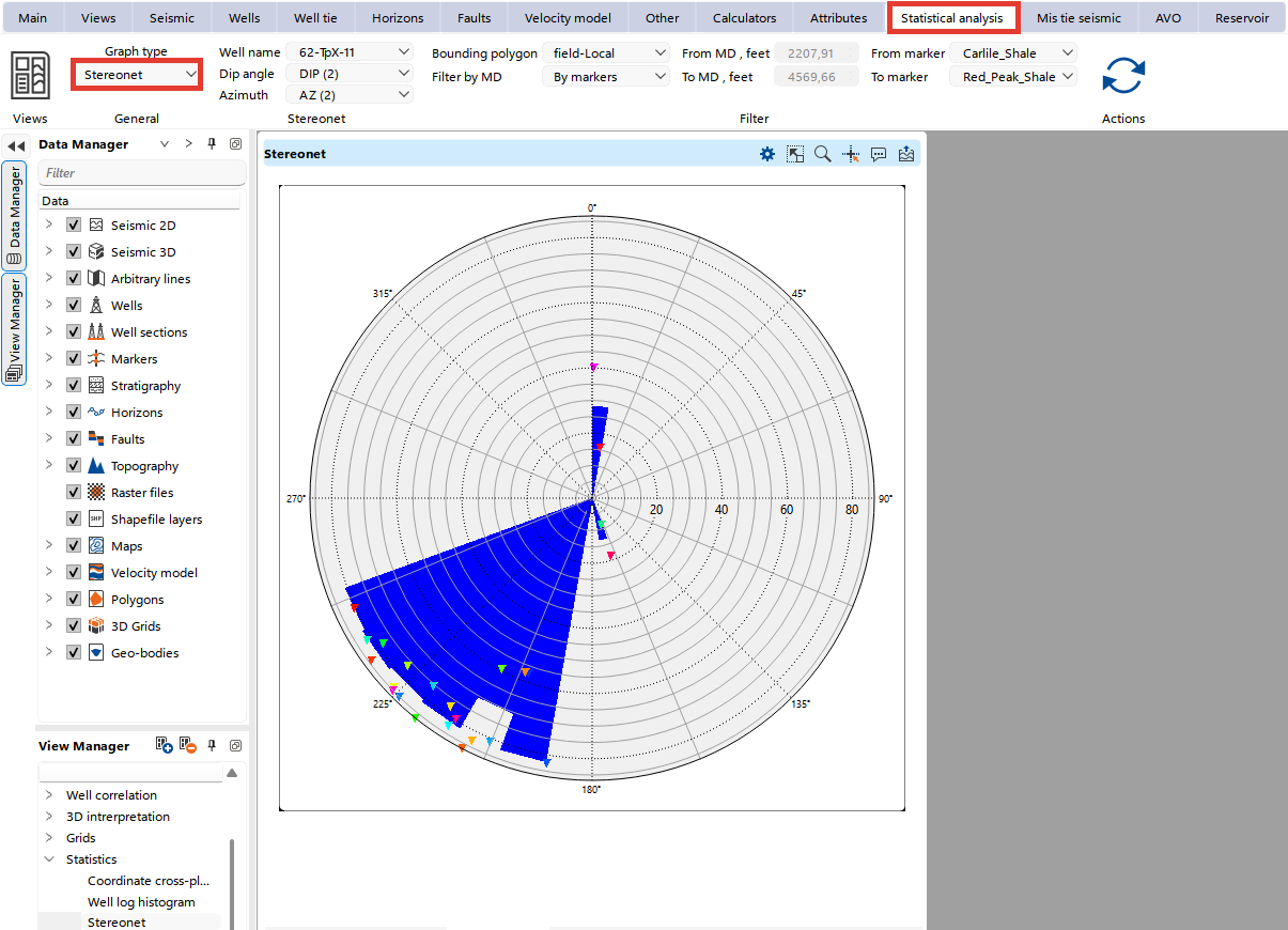
The Stereonet view is used to visualize the orientation of structural data, such as dip and azimuth, on a stereographic projection.
Well Name: Select the well to be analyzed.
Dip Angle: Choose the well log parameter for dip.
Azimuth: Select the well log parameter for azimuth.
Bounding Polygon: Limit points displayed on the cross-plot using a predefined polygon.
Filter by MD/Markers: For well data, filter points within specific measured depth (MD) ranges or between selected markers.
 click Update to see updated results after changing settings.
For more information about the cross-plotting please refer to Statistical analysis