AI Faults Wizard is a tool for automatic fault detection in 3D seismic data using neural networks. The wizard performs a complete processing cycle: from fault detection to generation of geometric objects ready for interpretation and analysis.

Purpose

The tool is designed for:

• Automating fault detection in seismic data
• Accelerating structural features interpretation
• Improving quality and detail of fault mapping
• Reducing subjectivity in manual interpretation

Features

• Automatic fault detection using trained neural networks
• Calculation of planarity (reflector continuity) and faultness (fault centerline) attributes
• Determination of fault orientation in space
• Generation of fault geometry (fault sticks) with automatic clustering into faults
• Preset parameters for quick start

Workflow

The wizard includes three sequential steps (tabs):

1. AI Fault Attribute — fault detection using neural network
2. Attribute Processing — calculation of planarity and fault characteristics (faultness and orientation)
3. Sticks & Faults — fault geometry construction

Requirements

• 3D seismic cube in SEGY format loaded into the project
• Seismic data available in Data Manager
• Sufficient RAM for cube processing

Launching the Wizard

Launch methods:

• Through Wizards panel (if activated)
• Through Ribbon menu → Faults → AI Faults Wizard

The wizard opens as a dialog window with three tabs (AI Fault Attribute, Attribute Processing, Sticks & Faults). Each tab contains parameters for the corresponding processing stage.

Results:

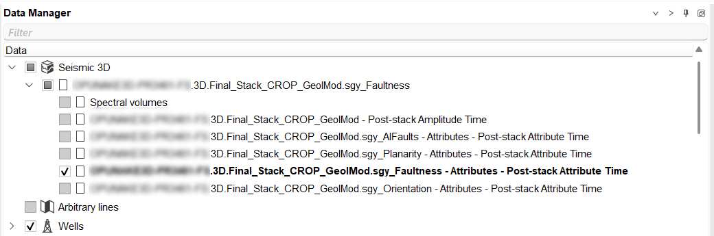
• All calculated attributes are automatically saved in Data Manager in the Seismic Data / Attributes section
• Each attribute is assigned a suffix for identification: _AIFaults, _Planarity, _Faultness, _Orientation
• Visual indicators (green checkmark) show successful stage completion
• Results from one step automatically become available for selection in the next step

Step-by-Step Guide

AI Fault Attribute Tab: Fault Detection

Application of a trained neural network for automatic fault detection in seismic data. The neural network analyzes fracture patterns and creates a probability map of fault presence.

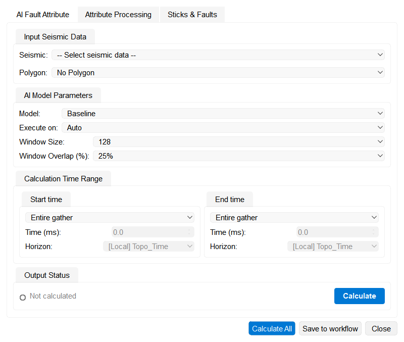
Procedure:

1. Select input data

• In Seismic:, select an available 3D seismic cube. Two-dimensional data is not supported.
• In Polygon:, select No Polygon to process the full volume, or select an available polygon to restrict the attribute calculation, sticks and fault surfaces to that area.

2. Configure AI model parameters

Model: selects the trained network used to estimate fault probability:

• Baseline — the default model. It accepts every listed Window Size, so you can trade local detail and processing cost against broader structural context.
• Transformer — an alternative trained model with a fixed Window Size of 128. Selecting it sets and disables the window-size control.

Note: Both models produce fault-probability attributes rather than interpreted fault objects. For a new dataset, compare their results on a representative polygon and use the model that best preserves the target fault patterns before processing the full volume.

Execute on: controls the processing device:

• Auto — tries NVIDIA GPU acceleration when it is available and falls back to CPU if GPU startup fails (default)
• CPU — runs on the processor
• NVIDIA GPU — explicitly requests GPU acceleration; if it is unavailable, the warning offers actions such as running on CPU or opening gInstaller

Window Size: is the seismic cube window supplied to the model:

• 32 — smallest local context and lowest processing cost
• 64 — a larger local context with moderate processing cost
• 128 — default for Baseline and the fixed value for Transformer
• 192 — broader structural context with greater time and memory use
• 256 — broadest available context and greatest processing cost

Window Overlap (%): is the overlap between adjacent windows:

• 0% — fastest, with the greatest risk of visible window boundaries
• 10% — limited boundary smoothing with a small processing increase
• 25% — default balance between smoothing and processing cost
• 50% — greatest boundary smoothing and highest processing cost

Calculation Time Range

Use the separate Start time and End time selectors to restrict detection to a vertical interval. Each selector has these modes:

• Entire gather — no limit at that end of the trace
• Time — use the fixed value entered in Time (ms)
• Horizon — follow a time horizon selected from the project-dependent Horizon: dropdown

Leave both selectors at Entire gather to process the full trace length.

3. Run calculation

• In the Output Status group, press the Calculate button
• Processing may take from several minutes to several hours depending on cube size and parameters
• Result is automatically saved in Data Manager with suffix _AIFaults
• After completion, a green checkmark and the calculated attribute name appear in the Output Status group

Result:

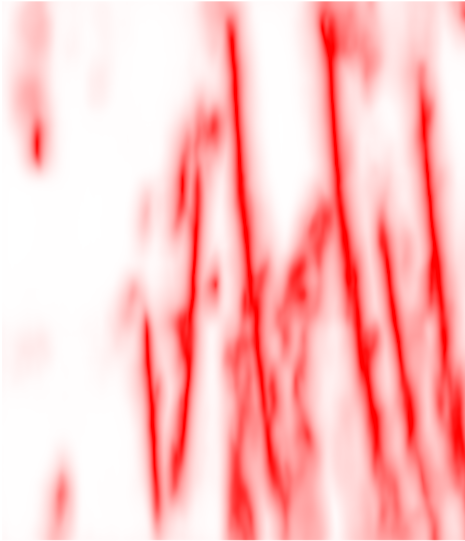
AI Faults attribute (SEGY format) — probability map of fault presence, where high values correspond to areas with high fault probability.

Attribute Processing Tab: Attribute Processing

Calculation of planarity and fault characteristics attributes. The tab contains two processing stages.

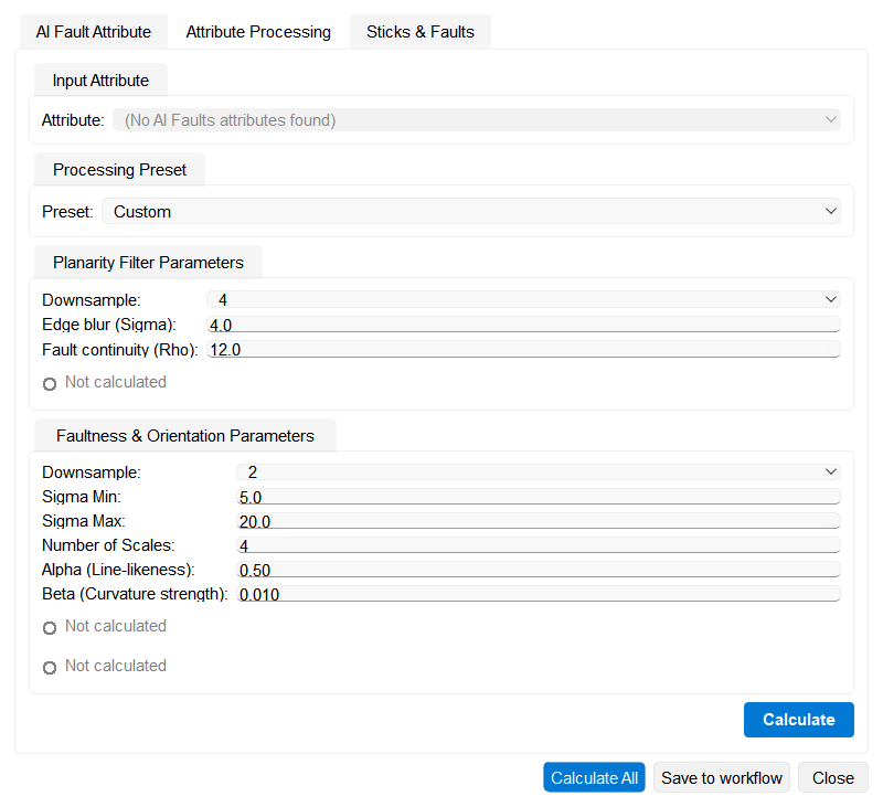
Processing sequence

The tab first calculates Planarity, a measure of seismic-reflection continuity, and then uses that result to calculate Faultness and Orientation. Faultness highlights a fault centerline for stick construction; Orientation records its horizontal direction.

1. Select an attribute

• The Attribute: dropdown lists available AI Faults attributes.
• The result from the AI Fault Attribute tab is selected automatically; choose another compatible attribute when required.

2. Select a processing preset

The single Preset: dropdown in Processing Preset controls both the planarity and faultness/orientation calculations:

• Sharp — limits smoothing for clear, well-defined faults
• Balanced — default starting point for general data
• Smooth — increases smoothing for noisy data or weak fault responses
• Custom — exposes all parameters in both groups for manual tuning

Note: Start with Balanced. Compare Sharp and Smooth on a representative area when boundaries are respectively clear or noisy; use Custom after inspecting those results because its controls affect both continuity filtering and fault-centerline extraction.

With Custom, configure:

• Planarity Filter Parameters — Downsample: 1, 2, 4, 6 or 8; higher values reduce processing time and resolution
• Edge blur (Sigma): smoothing scale used when detecting edges
• Fault continuity (Rho): neighborhood scale used to evaluate structural continuity
• Faultness & Orientation Parameters — Downsample: 1, 2, 4, 6 or 8
• Sigma Min and Sigma Max: lower and upper smoothing scales
• Number of Scales: number of scales included in the multi-scale calculation
• Alpha (Line-likeness): sensitivity to line-like structure
• Beta (Curvature strength): sensitivity to curvature strength

Note: Use lower Downsample values to retain detail and higher values for quicker trials. Wider smoothing and continuity scales can stabilize noisy responses but can suppress local changes, so compare Custom settings on a small area before a full-volume run.

3. Run the calculation

• Press Calculate. The wizard calculates Planarity first, then Faultness and Orientation.
• The results are saved with _Planarity, _Faultness and _Orientation suffixes.
• Status indicators show the result of each calculation.

Results:

• Planarity attribute (SEGY) — planarity map
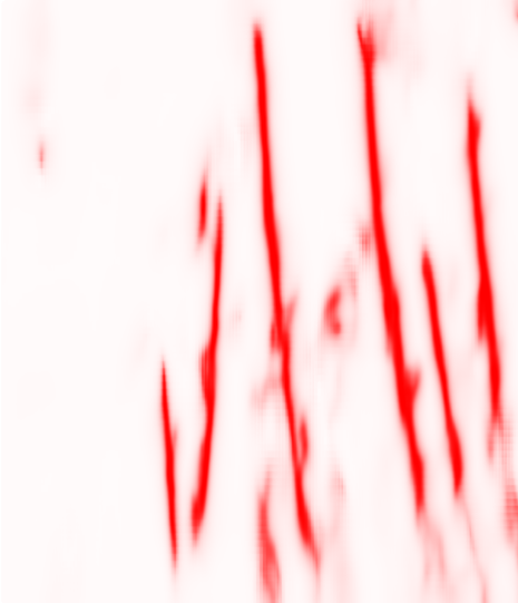
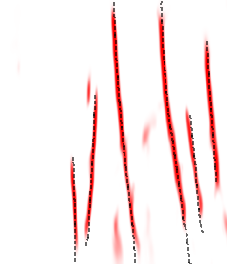
• Faultness attribute (SEGY) — fault centerline (ridge)
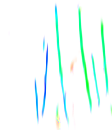
• Orientation attribute (SEGY) — fault strike azimuth in map view

Sticks & Faults Tab: Fault Stick Generation

Construction of three-dimensional fault geometry (fault sticks) based on fault centerline (Faultness) and orientation (Orientation) attributes. Faultness highlights the fault axis (ridge), allowing automatic stick construction along the centerline.

Process consists of two stages:

1. Stick tracing — construction of vertical lines along fault central axes. Each stick extends while the fault remains pronounced (high Faultness) and the fault strike azimuth does not change more than the tolerance (Orientation Tolerance).
2. Grouping into faults — for each stick in each time slice, the algorithm searches for neighbors in two directions along the fault strike (along the high Faultness line). Sticks are combined into one fault only if they are mutual neighbors: if stick A sees stick B on the left, then stick B must see stick A on the right. This prevents erroneous merging at fault branches.

Procedure:

1. Select attributes

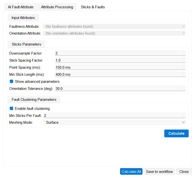
• In the Input Attributes group, select the fault centerline attribute (Faultness) and orientation attribute (Orientation) from the Fault Attributes stage
• Both attributes are selected automatically if the Attribute Processing tab is completed

2. Configure parameters

In the Sticks Parameters group:

• Downsample Factor: reduces resolution for faster processing; 1 keeps full resolution
• Stick Spacing Factor: sets spacing as a multiple of fault thickness; 1.0 means the spacing equals the thickness
• Point Spacing (ms): sets the distance between points along a stick; 0 keeps all points
• Min Stick Length (ms): excludes shorter sticks
• Show advanced parameters: displays Orientation Tolerance (deg)
• Orientation Tolerance (deg): sets the maximum direction change allowed while extending a stick

In the Fault Clustering Parameters group:

• Enable fault clustering: groups connected sticks into faults; clear it to retain free sticks
• Min Sticks Per Fault: sets the minimum group size; smaller groups remain orphan sticks
• Meshing Mode — Surface: reconstructs a continuous surface mesh
• Meshing Mode — Sticks: represents faults as individual stick lines

Note: Higher downsampling or wider stick spacing is useful for faster trials but reduces geometric detail. Increase the minimum stick length to suppress short fragments; increase Orientation Tolerance only when valid curved faults are being broken into separate sticks.

3. Run calculation

• Press the Calculate button (at the bottom of the tab)
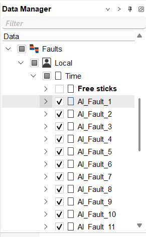
• Results are automatically added to Data Manager (Faults / Time or Depth)

Result:

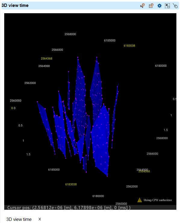
Fault Sticks — three-dimensional fault geometry represented by a set of vertical lines (sticks), grouped into individual faults. Available for:

• Visualization in 3D View, Map View, Seismic Sections
• Conversion to Surface Mode (fault surfaces)
• Export to other applications
• Further editing and interpretation

Calculate All

The Calculate All function performs all three steps sequentially in automatic mode — from fault detection to geometry generation. This is the most convenient method for complete processing.

Procedure:

1. Go to the AI Fault Attribute tab and select the seismic cube
2. Review and configure parameters on all three tabs (or leave defaults for quick start)
3. Press the Calculate All button (at the bottom of the wizard window, next to the Close button)
4. The wizard will automatically execute all stages in correct sequence

Advantages:

• Time saving: No need to manually switch between tabs
• Reliability: Automatic transfer of results between stages
• Convenience: Ideal for first run with default parameters

Save to workflow

After configuring the inputs and parameters, click Save to workflow to store the current wizard settings as a workflow task. Saving does not run the calculation; the task can be opened or executed later from the workflow.

Visualization of Results

Viewing Attributes:

After executing AI Fault Attribute and Attribute Processing, attributes are available in Data Manager → Seismic Data / Attributes. Attributes can be visualized in 2D/3D Seismic Views.

Viewing Fault Sticks:

Sticks & Faults results are available in Data Manager → Faults / Time (or Depth). Visualization options: 3D View, Map View, Seismic Sections. Mode switching: Free Sticks or Surface Mode. Display settings in Visual Settings (color, thickness, transparency).

Recommendations

General Approach:

• Start with Preset=Balanced for first run
• Use Calculate All for automatic execution of all steps
• Follow iterative approach: quick assessment → result analysis → detailed processing
• Use polygons to limit processing area for parameter testing

Performance Optimization:

• For a quick Baseline assessment, use Window Size 64 and Window Overlap 10%; Transformer always uses Window Size 128
• Use Downsample=2 or 4 on large cubes
• Increase Stick Spacing Factor to 2.0-3.0 for preview calculations

Quality Improvement:

• Check seismic data quality (structural smoothing can improve results)
• For clear faults: use Preset=Sharp with minimal smoothing
• For noisy data: use Preset=Smooth with increased regularization
• For curved faults: increase Orientation Tolerance to follow fault bends in horizontal plane

See Also

• Fault picking
• Seismic attributes
• Data Manager
• Import faults
• Export faults