ML Log Prediction is a machine-learning wizard that trains a model on existing well logs and then uses it to predict a missing or target log across other wells. The model is a gradient-boosted decision tree (CatBoost), and several models can be created, evaluated, and stored within a single project.

The wizard is organised into three tabs — Training, Analysis, and Calculation — that follow the natural workflow: build a model, check its quality, then apply it to generate predicted curves.

Purpose

The tool is designed for:

• Filling gaps where a log is missing in some wells but present in others
• Reconstructing a target curve from other available logs
• Building reusable prediction models that can be applied to all wells in a project
• Quality-controlling predictions through feature-impact and cross-correlation analysis

Requirements

• Wells with well logs loaded into the project and available in the Data Manager
• One or more input curves (predictors) and a target curve with valid samples in the selected training well or batch
• Matching curve names or mnemonics across wells so that the selected predictors and target can be found
• The CatBoost training engine. If it is not installed when the wizard opens, g-Space asks whether to download and install it; internet access is required for that download. If installation is not completed, the wizard closes.

Launching the wizard

Open the Petrophysics ribbon bar and click ML Log prediction. The wizard opens as a dialog window titled ML Log Prediction with three tabs: Training, Analysis, and Calculation.

Step-by-Step Guide

Work through the tabs in order: first train and save a model on the Training tab, review its quality on the Analysis tab, then apply it to wells on the Calculation tab.

Training Tab

The Training tab is used to create and train a model. Multiple models can be created and stored within a single project.

Training models — at the top of the tab, the Training models dropdown lists every model saved in the project. Its default entry is New training model. Select an entry to switch between models, or click the x button to delete the currently selected model (a confirmation prompt is shown).

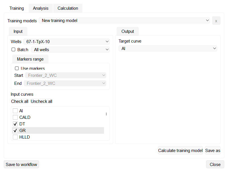
Input group — defines the training dataset:

• Wells — select one well. To train on multiple wells, enable Batch and choose All wells or an available filter, folder, or well section from the adjacent list.
• Markers range — enable Use markers to restrict training to the MD interval between the selected Start and End markers. When Use markers is cleared, the full log interval is used and the marker controls are disabled.
• Input curves — the checkable list of logs used as predictors. Use Check all or Uncheck all to toggle the whole list. At least one input curve is required.

Output group — set the Target curve: the single log the model will learn to predict. A target curve is mandatory for training.

Training and saving the model:

1. Click Calculate training model to train the model. On completion a message reports the model's MAE, RMSE, and prediction correlation, and the Analysis tab is populated with the results.
2. Click Save as and enter a model name when prompted. The model must be saved before it can be used on the Calculation tab; saved models appear in the Training models dropdown and are stored with the project.

Analysis Tab

The Analysis tab provides model evaluation and quality control. It reflects the currently trained or selected model.

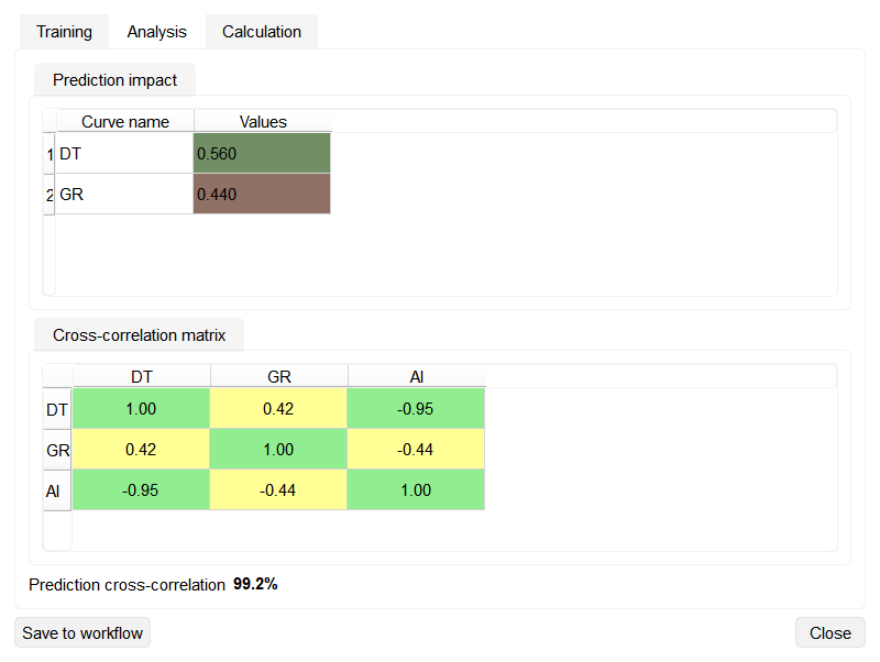
• Prediction impact — a table (columns Curve name and Values) showing how much each input curve contributes to the prediction, with a colour bar for quick visual comparison. Use it to identify the key predictors and to detect weak or redundant inputs.
• Cross-correlation matrix — the correlation between the input curves and the output curve, colour-coded by absolute correlation strength: green for strong, yellow for medium, and red for weak correlations.
• Prediction cross-correlation — a single performance indicator (for example 98.0%) expressing the agreement between predicted and actual values. It reads N/A until a model has been trained.

Calculation Tab

The Calculation tab applies a saved model to generate predicted logs.

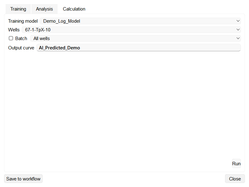
1. Choose a model from the Training model dropdown. Only saved models are listed.
2. Select one Wells entry, or enable Batch and choose All wells or an available filter, folder, or well section.
3. Set the Output curve name. The default is ML Curve 1, and it can be edited.
4. To save the configured prediction as a job instead of running it now, click Save to workflow; g-Space adds it to the current workflow. When you reopen that job for editing, Save updates it and Cancel closes without updating it.
5. Click Run to generate the predicted curves. A new log is written to each processed well and added to the Data Manager; a message reports how many wells were processed and how many, if any, failed.

Results

For every successfully processed well the wizard creates a new well log holding the model's prediction along the well's depth. The curve is saved to the Data Manager and can be displayed in the Well log view alongside the original curves. The completion message reports any wells that could not be processed.

Recommendations

• Choose input curves that are physically related to the target log, then use the Prediction impact table to drop weak or redundant predictors and re-train.
• Train only on wells that carry both the predictors and the target curve, and use a marker interval to focus the model on the reservoir section.
• Aim for a high Prediction cross-correlation and low MAE / RMSE before saving a model for production use.
• Create several models (for example per formation or per log type) and keep them in the project; the Analysis tab always reflects the currently selected model.
• Re-train and re-save a model whenever you change its input curves, target curve, or training wells.

See Also

• Petrophysics
• Porosity
• Saturation
• Shale Volume
• Well log calculator
• Workflows