Petrophysical Evaluation

The Petrophysical Evaluation wizard carries a complete well interpretation in one window instead of one calculator at a time. Its seven tabs follow the calculation order — 1. Environment, 2. Vsh, 3. PHI, 4. Saturation, 5. Permeability, 6. Matrix and 7. Results — and each tab consumes the results selected on the tabs before it.

Every method run produces a candidate curve. Several candidates of the same property can coexist, exactly one of them is selected, and only the selected curve is consumed further down the chain. Each computed curve is written to the well in the Data manager as soon as the run finishes, so results can be reviewed, displayed and exported from there. The wizard itself has no export step and never opens files: a curve that is not in the project yet has to be imported through the Data manager first.

Launching the wizard

Open the Petrophysics ribbon bar and click Evaluation in the Properties group. The command is named Petrophysical Evaluation and opens the window of the same name. The wizard is modeless, so the main window, the views and the Data manager stay available while it is open.

The wizard window

The top bar holds the Well list, the Interval label, the Run field that names the run (Base_Run_01 by default), the current environment version, the Mode list that switches between a deterministic and a stochastic evaluation, and the Save run and Recalculate chain buttons. Under it the numbered tab strip selects the step. Every step is laid out in three panes: the settings panel on the left, the depth track in the middle, and a tab-specific crossplot or QC panel on the right. Draggable dividers separate the three panes: drag one to give the settings, the depth track or the QC panel more room. No pane can be dragged away completely, the widths you set apply to all seven tabs, and they are restored the next time you open the wizard. Widening the window itself adds the extra space to the depth track and keeps the side panes as you set them. Run at the bottom of the window calculates the active tab, and Close closes the wizard.

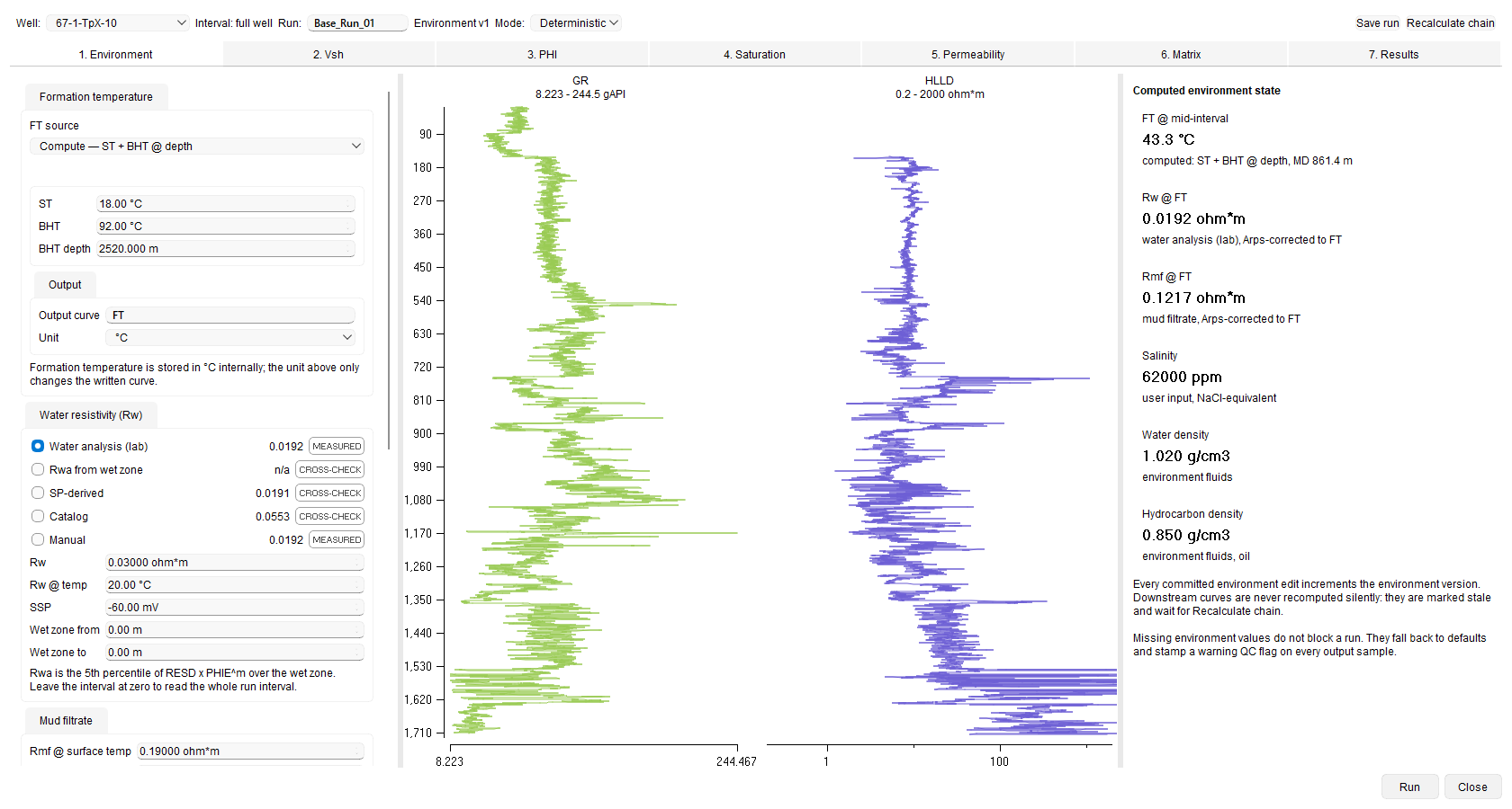
The depth track plots the curves of the current step against a shared measured-depth axis, and each lane is titled with the curve name, its scale and its unit. Selecting another well in the top bar clears the candidates, because they belong to the well they were computed for.

Candidates and selection

Tabs 2 to 6 keep a list of candidate curves. Each row carries a selection button, a colour swatch, the curve name, a PROJECT badge when the curve was taken from the project, and QC percentages for valid, warned and clipped samples.

Selecting a candidate – exactly one candidate per property is selected, and it is the one every downstream tab reads.
+ Run another method – calculates the method chosen in the adjacent list and adds it to the list as its own candidate. Running the same method again replaces its candidate.
Save as copy – freezes the current candidate under a copy name, so a later run of the same method can be compared against it.
Delete – removes a candidate. A candidate that a later tab has already consumed cannot be deleted; the wizard names the consumer and asks you to select another candidate and run again first.

Using a curve from the project

Instead of calculating a property, you can register a curve that already exists in the well — the output of another calculator, or log data imported earlier through the Data manager. Click Use from project... and complete the Use curve from project dialog:

Curve and Origin – the curve of the selected well and where it came from.
Declared as – what the curve is. For a porosity curve, Porosity type additionally states whether it is total or effective porosity, because that changes the calculations that consume it.
Curve unit and Interpret as – the unit stored with the curve and the unit it is read in.
Depth and Range – how the curve is resampled onto the depth step of the run, and which part of the interval it covers. Samples outside the range of the source curve stay undefined.

The registered curve becomes an ordinary candidate with a PROJECT badge, and its values are never modified. Because it does not depend on anything calculated inside the wizard, it never goes stale.

Staleness and Recalculate chain

Nothing is recalculated silently. When you change an input that a calculated curve consumed — for example a value on the 1. Environment tab — every curve that depends on it is marked stale, a banner names the affected steps, and the stale curves are drawn dimmed on the depth track. Recalculate chain re-runs only the stale steps, in dependency order, and reports which ones it recalculated; if nothing is stale it reports that as well. The only exception is dragging the endpoint lines on the 2. Vsh histogram, which recalculates that tab’s own candidates as you work.

Stochastic mode

The Mode list in the top bar switches the whole wizard between Deterministic and Stochastic. Deterministic is the default and works exactly as described above: every parameter is a single number. In Stochastic mode the parameters you gave an uncertainty distribution are drawn at random and the whole chain is run again for each realization, so the uncertainty of the shale volume reaches the porosity, the saturation and the permeability instead of stopping at its own tab. Switching back to Deterministic keeps the distributions you entered, and they reappear when you switch to Stochastic again.

Selecting Stochastic adds a second row to the top bar:

Realizations – how many parameter sets are drawn: 100, 500 or 1000.
Random seed – the number the draws start from. The same seed on the same inputs reproduces the run exactly, including after saving it and reopening the wizard; Regenerate replaces it with a new one.
Correlation – reads Off: the parameters are drawn independently of one another.
Save per-realization sensitivity dump – asks for a CSV file when the run finishes and writes one row per realization with the values that were drawn, so you can see which parameter drives the spread.

A small ± button and a summary appear beside every parameter that can carry a distribution, and both are hidden again in Deterministic mode. The summary reads Fixed until a distribution is set and afterwards names it with its minimum, mean and maximum. The ± button opens the Uncertainty dialog of that parameter, which offers Normal, Lognormal, Triangular and Uniform, each described by Min, Mean and Max; for the normal distribution the standard deviation derived from them, (Max − Min) / 6, is shown read-only under the fields. A parameter that has no distribution yet opens centred on the value the tab currently shows. OK stores the distribution and Set fixed removes it again; a minimum above the maximum is refused, and a mean outside the range is moved back into it.

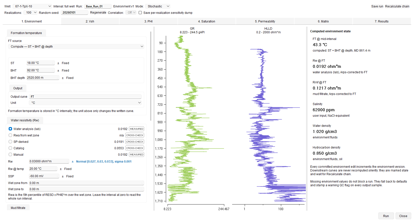
Distributions belong to the model parameters and not to the choice of method or source. They are offered on the surface and bottom-hole temperatures and the depth the bottom-hole temperature is read at, the temperature gradient, the measured water resistivity and its temperature, the static SP deflection, the mud-filtrate resistivity and its surface temperature and the salinity on 1. Environment; on the clean and shale endpoints of 2. Vsh; on the matrix and fluid densities, the matrix and fluid travel times, KCP, PHIDSH and PHINSH on 3. PHI; on the tortuosity factor, the cementation and saturation exponents, the shale resistivity and the shale porosity of 4. Saturation; on the coefficients of each permeability method, the bulk-volume-water constant and the manual irreducible saturation of 5. Permeability; and on the endpoints of every mineral on 6. Matrix. Limits and thresholds stay single-valued and are applied unchanged to every realization: the porosity clamp PHIMAX, the permeability Floor and Cap, and the cutoffs of 7. Results.

Run means the same thing on 2. Vsh, 3. PHI, 4. Saturation and 5. Permeability in this mode: it runs the complete chain once per realization and reports its progress in a Stochastic evaluation window. The mineral solve joins that run when 6. Matrix holds a solvable system, and the zone summation is repeated over the same realizations, so one run fills the whole wizard. 1. Environment, 6. Matrix and 7. Results keep their own single deterministic Run.

The run is checked before it starts. It needs at least one distribution that the selected methods actually use and a seed to start from, and the clean and shale windows on 2. Vsh must still keep the separation the driving log requires, distributions included; whatever is missing is named instead of run. Two candidates cannot be selected in this mode, because neither carries model parameters that can be sampled: one registered with Use from project..., and the Minimum of candidates (QC floor) curve. The wizard reports that when you switch modes and selects a computed candidate in its place, or asks you to compute one first.

While a stochastic run is loaded, the depth track of tabs 2 to 5 gains a shaded P10-P90 band for that property with the deterministic curve drawn over it as a dashed line, so the single answer can be read against the spread around it. On 2. Vsh the histogram also draws each sampled endpoint distribution over the bars: the solid line is still the endpoint and carries the mean of its distribution, the dashed lines beside it are its minimum and maximum, and all of them can be dragged. 6. Matrix reports under Log responses how many realizations had to be rescaled for the mineral volumes to close on one, with the mean excess over the interval; a large fraction means the endpoint distributions are wider than the closure condition can absorb.

7. Results replaces the zone summary with a percentile table: one row per summed quantity for each zone and for TOTAL, in the columns P90 (low case), P50 and P10 (high case), and Zone table → CSV exports it in that form. Because the cutoffs are not sampled, the spread reflects the parameters alone; the gross thickness of a zone does not depend on them and is therefore the same in all three columns.

Each family writes its percentile curves to the Data manager beside the deterministic ones, taking the mnemonic of the selected method and adding _P90, _P50, _P10, _MEAN and _SD; every mineral volume of a stochastic matrix solve gets the same set. The convention is the petroleum one and the completion message repeats it: P10 is the high case, the 90th percentile of the realizations, and P90 the low case, the 10th percentile. Editing a distribution, a parameter or an input afterwards marks the stochastic outputs stale in the same way the deterministic chain does, and Recalculate chain runs the realizations again.

The tabs

1. Environment

Sets the well conditions that the later tabs need, and calculates the formation temperature curve.

Formation temperature – FT source offers Compute — ST + BHT @ depth (the default, from a surface and a bottom-hole temperature at a stated depth), Compute — ST + gradient G and Use from project — existing FT curve. Switching between the two computed forms carries the equivalent values across. Under Output, Output curve names the result (FT by default) and Unit sets the unit it is written in; internally the temperature is always kept in degrees Celsius.
Water resistivity (Rw) – one active source out of Water analysis (lab), Rwa from wet zone, SP-derived, Catalog and Manual. Each row shows the value it produces and a MEASURED or CROSS-CHECK badge, and the fields below feed them: the measured Rw and its temperature, the static SP deflection, and the wet-zone interval the cross-check reads.
Mud filtrate – Rmf @ surface temp, Surface temp and Salinity.
Depth track – the GR curve and RESD curve to display. The deep resistivity curve chosen here is also the one that 4. Saturation requires.
Interval – the same depth-range selector as the other calculators on the bar (MD range, TVD range, TVDSS range, Markers range and Zones range), plus Step MD, the depth step every curve of the run is calculated on. Calculating all wells in one batch is not available in this wizard.

On the Zones range tab, tick one or more zones of a zone set to confine the whole run to those zones. The selection replaces the depth range set on the other tabs instead of narrowing it: every tab reads only the samples inside the selected zones, and the rock between two of them is left out of the calculations and of the summation. The top bar then reports the zone selection and the depth range it spans in place of the Interval label. A selected zone that has no interval in the current well is skipped and reported; if none of them resolves, the run stops and asks you to check the zone markers or to use another interval tab.

The right panel, Computed environment state, shows the resulting formation temperature at mid-interval, the water and mud-filtrate resistivities corrected to that temperature, the salinity and the fluid densities, each with the source it came from. Missing environment values never block a run: the calculation falls back to defaults and marks the output samples with a warning.

2. Vsh

Calculates the shale volume. Under Input, Log selects the driving log (GR, SP or RHOB-NPHI), Curve the curve that carries it, and Zone which part of the run the histogram is read on. The zone list follows the zones selected on the 1. Environment tab: its first entry is All selected zones — or Whole run interval when no zones are selected — followed by one entry per selected zone in depth order, and two zones that overlap appear as one entry carrying both names. Picking a zone scopes the histogram only: the clean and shale endpoints and the calculated shale-volume curve still cover every selected zone, and a hint under the row states that. Under Endpoints, the clean and shale values of that log are entered as numbers; a line below reports the current separation and the minimum the log requires, and warns when the methods are excluded because the endpoints are too close together.

The right panel is a histogram of the driving log with two draggable endpoint lines, clean and shale. Dragging a line updates its numeric field immediately and recalculates the candidates that use that log, so the endpoints can be picked visually against the data.

The available methods are Linear (IGR), Steiber, Clavier, Larionov, tertiary rocks, Larionov, older rocks and Minimum of candidates (QC floor). All but the linear index are calibrated on gamma ray, so the other logs offer the linear index alone. Selecting the minimum curve shows a warning that it is a quality-control floor rather than an interpretation, because the tabs that consume it inherit its optimistic bias.

3. PHI

Calculates porosity from the density, neutron and sonic curves selected under Input. Matrix and fluid sets the rock matrix (Sandstone, Limestone or Dolomite, which fills in the matrix density and travel time), the fluid density, the upper clamp PHIMAX and the compaction correction KCP. Shale correction holds the shale endpoints PHIDSH and PHINSH, which are applied together with the shale volume selected on 2. Vsh. Gas handling offers Auto — detect ND crossover (the default), Force liquid and Force gas.

The methods are Neutron-Density, Density, Neutron and Sonic (Wyllie). Each run writes three curves: the interpretation curve, an unclamped twin, and a flag curve that marks the samples the clamp changed. The right panel is a neutron-density crossplot with the sandstone, limestone and dolomite reference lines.

4. Saturation

Calculates water saturation. A read-only Consumes banner states which environment version and which selected porosity and shale-volume curves the run will use. The methods are Simandoux, Archie and Dual Water; a hint line reports the average shale volume over the interval and suggests a method for it, but never changes the selection for you. Electrical properties holds the tortuosity factor, the cementation and saturation exponents, the shale resistivity and the shale porosity; the last two reach the shaly-sand methods only, as Archie reads the first three alone.

This is the one step that cannot fall back to a default: without a deep resistivity curve the run stops and reports Select a RESD curve on the Environment tab before running Saturation. The right panel is a Pickett plot with the Sw = 1 (water line) and Sw = 0.5 overlays.

5. Permeability

Calculates permeability from the selected porosity and an irreducible water saturation. The methods are Timur, Morris-Biggs and Coates, each with its own group of coefficients.

Irreducible water saturation – SWirr source is either the Buckles relation, whose bulk-volume-water constant Fit BVW from the zone estimates over the interval you enter, or Manual constant.
Calibration – Target type records what the result is calibrated against: uncalibrated (the default), core — air K, core — Klinkenberg or core — liquid K. An uncalibrated run keeps a warning on its output.
Trimming – Floor and Cap bound the result in millidarcy, and the samples they change are flagged.

The right panel plots permeability against porosity on a logarithmic axis, with the trend line of the selected model.

6. Matrix

Solves the mineral composition of the rock from the log responses. The clay volume is not solved for: it is fixed to the shale volume selected on 2. Vsh, which is why the first row of Components is locked. The other rows are minerals taken from the shipped mineral table, with editable endpoints; + Add mineral adds another one and Custom mineral duplicates the mineral above it under an editable name.

Log responses selects which measurements enter the solve — RHOB, NPHI, PE and DTC — on top of the closure condition, which is always present. A counter reports how many equations and unknowns the current setup has and whether the system is square, underdetermined or overdetermined. While there are more unknowns than equations, Run is unavailable and the counter asks you to add a response or remove a mineral. Non-porous pre-solve triggers can additionally recognise halite and anhydrite intervals from their log fingerprint before the solve runs.

The run writes one volume curve per component plus a closure-residual curve, and the depth track shows the components stacked to a full section. The right panel is a matrix-density against matrix-cross-section crossplot with the quartz, calcite and dolomite triangle; samples inside it are feasible three-mineral mixtures.

7. Results

Applies cutoffs to the selected curves and sums the interval. An Inputs consumed line lists the curves and the environment version the summation reads. The cutoff set holds VSH_MAX, PHI_MIN, SW_MAX, PERM_MIN and MIN_BED_THICKNESS, and Run summation applies them. An Averaging group states the conventions the summary uses, so the basis of every number is visible.

The right panel is the zone summary table. It holds one row per zone selected on the 1. Environment tab — or a single ZONE_1 row over the whole interval when no zones are selected — followed by a bold TOTAL row. Its columns are Zone, Gross m, Net Res m, Net Pay m, N/G, the average porosity over the reservoir and over the pay, Sw avg, the oil saturation coefficient, the geometric mean permeability and HPV m. The run writes the net reservoir and net pay flag curves to the Data manager. Zone table → CSV saves the table as a CSV file; run the summation first, otherwise the wizard asks you to.

Saving and reopening a run

Save run in the top bar and Save run snapshot on the 7. Results tab do the same thing: they run the summation and store the state of the run on the flag curves it writes, so that a saved run always matches numbers that were actually calculated. Reopening the wizard on the same well restores the candidates, the selections, the parameters and the zone table of that run. In Stochastic mode the snapshot also carries the mode, the realization count, the seed and the whole distribution table, so a reopened run is set up to reproduce itself; a run saved before the mode existed reopens as Deterministic.

In the Data manager, right-clicking a curve that carries a saved run — the net reservoir and net pay flags, and the percentile curves of a stochastic run — offers Show evaluation settings, which opens the wizard on that well with the stored run restored.

There is no separate save step for the curves themselves. Every run writes its outputs to the well immediately and reports which curves it wrote, and they appear in the Data manager tree straight away. Exporting them to LAS, like importing new log data, is done from the Data manager.