The Mohr diagram view shows the fracture planes of a well core table against a single stress state, so that the planes which are close to slipping can be told apart from the ones that are not. Every plane is drawn at its own effective normal stress and shear stress, together with the Mohr circles of that stress state and a failure envelope.

To create a Mohr diagram view go to the Views bar, navigate to Graphs and click on Mohr diagram. Each click opens a diagram of its own, with a stress state of its own, so the same core table can be examined under several stress states at the same time. The view stays empty until a core table has been selected.

Fracture planes

The planes are read from a table in the Core > Tables folder of a well. Where the picks are not in the project yet, right-click the well or its Core folder in the Data manager and choose Import core data > Tables... to read them from a file. The columns that carry strike, dip and dip direction are chosen in the view rather than on import, so tables whose headers come from different interpretation packages can be used without renaming a column.

Choosing the data

The diagram is set up on the Statistical analysis bar: choose Mohr diagram in the Graph type list of the General group, then fill in the Mohr diagram group.

• Core table - the well core table that holds the fracture picks.
• Strike, Dip and Dip direction - the columns that carry the orientation of each plane, in degrees. Nothing is drawn until all three have been chosen.
• Aperture and Type - optional columns. They take no part in the calculation and are used only to colour and to size the points.
• Reference depth - the depth the stress state applies to. One stress state is used for the whole population.
• Stress unit - psi or MPa, used by both axes and by every stress field. A table measured in feet belongs with psi and a table measured in metres with MPa; a mismatched pair is refused rather than computed, and the reason is written in place of the horizontal axis title.
• Sv source, Sv curve and Sv - the overburden stress. Keep Manual and type the value, or choose Well curve and pick an overburden stress curve of the core table's own well; the value is then read at the reference depth and shown in Sv.
• Pp source, Pp curve and Pp - the pore pressure, entered in the same two ways.
• SHmax, Shmin and SHmax azimuth - the two horizontal stresses and the direction of the larger one, in degrees from north. An azimuth outside 0-360 degrees is refused.
• Faulting regime - Auto takes the largest of the three magnitudes as S1 and the smallest as S3. Choose Normal, Strike-slip or Reverse where the automatic choice is not the intended one, which happens when two of the magnitudes are close.
• Friction mu - the friction coefficient the failure envelope is drawn with, 0.6 to begin with.
• Show S1-S2 circle and Show S2-S3 circle - the two inner circles, drawn to begin with. The outer S1-S3 circle is always drawn.
• Reference envelopes - adds dashed envelopes at mu = 0.6 and mu = 1.0, which bracket the range friction usually takes in rock, on top of the envelope at the chosen friction coefficient.
• Colour by - what the colour of a point carries: Slip tendency to begin with, or Aperture, Depth or Type. Aperture and type need the matching column chosen above.
• Size by aperture - the size of a marker follows the aperture column.
• Critically stressed only - keeps only the planes of the critical band, both in the plot and in the table. The reported counts still describe the whole population, so what the diagram says does not change with it.

In the Filter group, set Filter by MD to Manual and enter From MD and To MD to narrow the diagram and the table to a depth window. Left at Not required, the whole table is used.

Every one of these controls redraws the diagram at once, so the Update graphs button is not needed here. Varying Friction mu and watching which planes cross the envelope is the main use of the view.

Reading the diagram

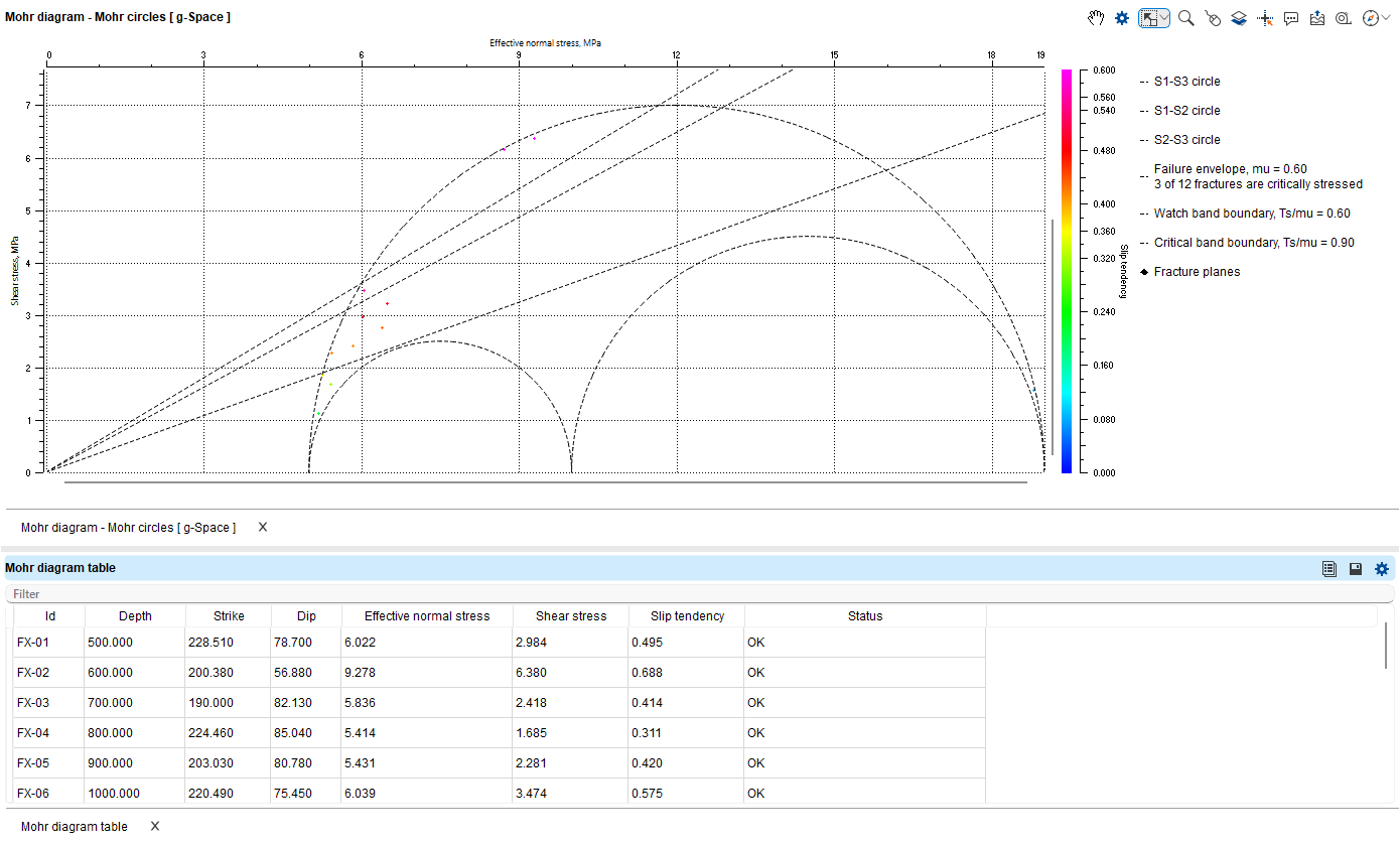
The horizontal axis is the effective normal stress and the vertical axis the shear stress, both in the chosen stress unit. The two axes are kept at the same scale, so the circles stay circular through zoom and pan and the slope of the envelope can be judged against them.

Three circles centred on the horizontal axis bound the stress state: the outer S1-S3 circle and the inner S1-S2 and S2-S3 circles. A plane belongs inside the outer circle and outside the two inner ones; one that falls elsewhere points at an input or a stress state to be checked, and it is drawn rather than cut away.

The failure envelope is the dashed line from the origin whose slope is Friction mu. Each plane is a point coloured by its slip tendency, with the colour bar beside the plot. The legend names the circles, reports the envelope with its friction coefficient and the number of fractures that are critically stressed, and marks the boundaries of the watch and of the critical band. Where some rows could not be plotted or carry a flag, it also reports how many rows are in the depth range, how many are plotted, how many are only listed and how many are flagged.

Result table

The Mohr diagram table under the plot lists the same planes, with Id, Depth, Strike, Dip, Effective normal stress, Shear stress, Slip tendency and Status. Every column can be sorted, which brings the planes closest to slipping to the top. Pointing at a point highlights its row and pointing at a row highlights its point, and a row can also be selected by clicking it. The depth filter applies to the table exactly as it does to the plot.

Status reads OK for a plane with nothing to report. Otherwise the row is shaded and the column names what was found: angles that could not be read, angles outside their range, a dip direction that disagrees with the strike, a depth outside the logged interval of the well, or an effective normal stress of zero or less. A flagged row is always listed and never dropped, so the rows in the table account for every row of the core table in range. A plane whose effective normal stress is not positive has no slip tendency, and it is not presented as a stable one.

Stability bands

Every plotted plane falls into one of three bands, taken from the ratio of its slip tendency to the friction coefficient: stable, watch and critical. Three bands are used rather than a plain yes or no because the stress magnitudes, the azimuth and the friction coefficient all carry uncertainty.

The two limits are 0.60 and 0.90 to begin with, and they are set once for the whole application rather than per diagram: open the Tools menu, choose Options ... and use Watch band starts at Ts/mu and Critical band starts at Ts/mu in the Mohr diagram stability bands group of the General tab. The critical limit is kept above the watch limit. Open diagrams are recoloured as soon as the values are changed, and a saved diagram is reopened with the limits that are configured at that time.

Saving and exporting

Right-click the plot to open the context menu of the view:

• Save Mohr diagram to Data Manager... - asks for a Name and stores the diagram in the Mohr diagram folder of the Statistics category of the Data manager. Opening it again restores the core table, the column choices, the stress state, the friction coefficient and the filters. A name that is already used in that folder is refused.
• Export Mohr table to CSV... - writes the listed planes to a CSV file, with the depth and the orientation of each plane and with the computed effective normal stress, shear stress, slip tendency, its ratio to the friction coefficient and the band. Where the filters leave nothing to write, the view reports that instead of writing an empty file.