Wells - contains any type of well data

A Wells folder can hold well headers, inclinometry, logs (LAS / DLIS files, one-dimensional curves and array channels), markers, checkshots, comments, core data and rasters/images.

Right-click the Wells icon in the Data Manager to access:

• Import (Checkshot, LAS / DLIS files, Rasters, Core data > Tables... / Images..., WITSML, PRODML, Well headers, Well headers from IHS 297 fixed files, Well headers from Petrel, OSDU data model...)
• Export (Wellheads, Inclinometry, Checkshot, LAS)
• Create empty well
• Manage custom log types...
• Scale curves
• Extract seismic trace (for all wells in the folder)
• Log Mode (Curves / LAS files)
• Clear checkshot
• Clear LAS files
• Clear wells
• Sort by name
• Add folder

Wells can be grouped in folders under Wells; use Add folder to create one. Right-click a well folder to run Extract seismic trace for every well below it, wells in nested folders included, to open its Export submenu, or to Remove those wells. On the Wells folder itself, Extract seismic trace is unavailable until the project contains at least one well.

When the project is connected to a database, additional actions are available according to your permissions:

• Receive wells
• Commit wells
• Receive checkshots
• Commit checkshots
• Receive las
• Commit las

Deleting well data

Commands that delete well data ask you to confirm first. Clear checkshot, Clear LAS files and Clear wells on the Wells folder, and Remove, Clear markers, Clear LAS info and Clear checkshots on an individual well, open a Confirm message that names the data to be removed. Click Yes to delete it or No to keep the data; No is preselected. The same confirmation appears when you remove several selected wells, LAS files or log curves at once, and for the Clear wells inclinometry and Clear all wells comments commands on the Wells bar.

Log Mode

Log Mode controls how the logs of every well are arranged in the Data Manager. Right-click the Wells folder, point to Log Mode and choose Curves or LAS files; the mode currently in use is checked. The same setting is available from the Log Mode drop-down on the Wells bar.

Curves is the default mode and the arrangement the rest of this topic assumes: under each well, Logs and the user item below it list the log curves under the names you gave them, curves that belong to a LAS set are grouped in a folder named after that set, and the Wells branch starts with the global All curves section.

In LAS files mode, each imported LAS file appears as its own item under Logs and the user item, named after the file without its extension, and the curves it contains are listed inside it. Those curves are labelled with the original mnemonic read from the LAS file rather than the name you gave them, so a curve you renamed to Gamma Ray 1 is listed as GR. The index curve of the file comes first as MD, the remaining curves follow in alphabetical order, and two extra columns to the right of each curve show its type and its units. LAS set folders and the global All curves section are not shown in this mode.

Multi-dimensional array channels imported from DLIS are also listed in both modes. A file containing only array channels still has a Logs branch under its well. In Curves mode they appear by name below their user, and channels from editable files also appear in All curves; they do not go inside LAS set folders. In LAS files mode each channel remains below its source file, with its kind and units in the two additional columns.

Switching the mode only re-arranges how the logs are listed - no curve, name, type or file is changed - so you can switch back and forth freely.

Curve colours

You can give each log its own colour in the Data Manager. Right-click All curves, or one of the LAS set folders under it, and choose Colorize to give every curve name in that scope a distinct colour. Right-click a single curve under All curves and choose Set color to pick its colour yourself, or Colorize to have one assigned automatically. You can also select several curves - under All curves or under a well's Logs list - and use Colorize on all of them at once. A single curve listed under a well has no colour command of its own.

The colour is stored with the project against the curve name, so the same log name keeps that colour in every well, and it is shown as the background of the curve icon in the Data Manager.

In well log views the colour is used as the default colour of that curve, and views that are already open are redrawn. A colour saved in a well template and a colour set for the curve in the view's Curve Settings both take precedence over it.

Displaying LAS curves

With a well log view active, select a log curve's checkbox in the Data Manager to add it to the active track. If the well has no active track, a new track is created. Clear the checkbox in the Data Manager to remove the curve from every track in the well log view. Selecting the checkbox again returns the curve to the track or tracks it was removed from - to several tracks at once when it was displayed on more than one - but a track deleted in the meantime is not recreated, and when none of the remembered tracks is left the curve is added to the active track as described above. The placement is remembered while this view stays open and is not stored in the project. This works for curves under an individual well and, in Curves mode, for the global logs under All curves.

To change one track only, right-click the track, choose Advanced Track Settings..., and select or clear the curve in the Curves section. This does not add or remove the same curve on other tracks.

With a time- or depth-domain 3D view active, select a LAS curve's checkbox in the Data Manager to display the curve along its wellbore; clear the checkbox to hide it. A synthetic trace saved as a LAS curve can be displayed in the same way.

To change its 3D appearance, open Visual Settings, select the curve under Las curves 3D on the Object(s) tab, and adjust Curve style, Line color, Line size, and Gain.

Displaying checkshot curves

Every checkshot loaded on a well is listed under Checkshot in the Data Manager, and each checkshot holds two curve items, TWT and Vint, with the same checkbox as any other object. Only the checkshot currently in use for the well - the one shown in bold - supplies the curves that can be displayed.

With a well log view active, select TWT or Vint to add that curve to the active track; if the well has no active track, a new track is created. Clear the checkbox to remove the curve from the view.

The same checkboxes also show and hide these curves along the wells drawn on inline, crossline and arbitrary line seismic sections, in time and in depth, where the display additionally follows the Show las curves on seismic views property described in Module Properties. In a 3D view only LAS curves are drawn along the wellbore.

Core data

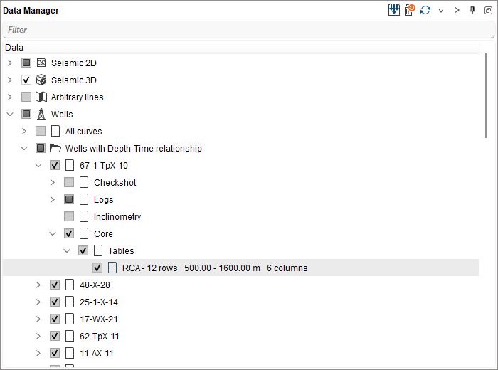
Core measurements are kept with the well they were taken from. As soon as a well holds core data, a Core folder appears under it in the Data Manager, beside Logs and Checkshot; a well with no core data has no such folder. Core is grouped inside it by the shape it arrives in: Images holds core photographs registered to a depth interval, Tables holds plug and sample measurements with one row per sample, and Curves holds continuous measurements along the core. Each sub-folder is shown only when the well has that kind of core data.

Every item carries a summary beside its name, so it can be recognised without being opened: an image shows its kind and depth interval, a table shows its number of rows, its depth range and its number of columns, and a curve is marked as core and shows its unit, depth range, sampling step and depth reference. Depths are stored exactly as they were read - nothing is converted or shifted on import.

Right-click Core and choose Properties for a summary of the folder: the depth unit of its core, whether the depths are on core depth or on log depth, and how many tables, curves and images the well holds, with the space those images take in the project.

To bring core data in, right-click the well, point to Import core data and choose the entry that matches what the file holds:

• ASCII files... - a continuous core measurement, which becomes a curve under Core > Curves.
• Tables... - a lab spreadsheet of plug or sample measurements, which becomes a table under Core > Tables.
• Images... - core photographs, which become images under Core > Images.

The same Import core data menu is on the Core folder, and each sub-folder offers only the entry that fills it. The entry is chosen by what the data is, not by the type of the file, so Tables... and ASCII files... read the same kinds of column file. When the file clearly does not fit the entry that was chosen - a reading every centimetre is not a plug table - a message says so and offers to import it through the other entry instead.

Core tables

Import core data > Tables... accepts a *.csv, *.txt or *.xlsx file and opens the Import core table dialog, which states what every column of the file means before anything is stored.

• 1. File - the file being read. The separator and the row the table starts on are detected and reported under the fields; correct Separator, The table starts with a row of column names or Table starts at row when the detection is wrong.
• 2. Preview (the file exactly as it is) - the first rows of the file as they are written, before anything is interpreted.
• 3. Columns - what each column is. Set Column is to Depth for exactly one column, and to Depth to, Well id, Sample id, Property or Ignore for the others. A Unit has to be typed for every numeric Property column - units are never guessed, and the import names the columns that are still without one.
• 4. Depth and empty values - the Depth unit, whether Depth is Core depth or Log depth, and the No value text (-999.25 by default) whose cells are stored as empty. Enable Fill down depth to copy the preceding numeric depth into blank rows within the same well/sample block. It never replaces present nonnumeric text or carries a depth into a new block; blanks before the first depth in a block remain empty. The option is unavailable when every row already has a depth.
• 5. Where it goes - the Well the core belongs to and the Table name it is stored under; the name of the file is offered.

Read the status below Fill down depth before importing. It either reports the rows and well/sample blocks that can be filled, or confirms Every row carries its own depth.

Import stores the table and reports how many rows were read and kept, how many columns were kept, the depth range and, when applicable, how many blank depth cells were filled. A row is left out only when its depth remains empty or does not hold a number after optional fill down, and every row left out is listed with the reason. Two rows at the same depth are both kept, so a horizontal and a vertical plug from the same sample stay two separate measurements.

Right-click a core table to Open it in the table editor, to Rename it or to Remove it. New table on the Tables folder asks for a name and opens the same editor on a starter grid of a Depth, a Sample and a Property 1 column with five empty rows, for a short description typed in from a report. In the editor, type into the cells and shape the table with Add row, Delete row, Add column... and Delete column; double-click a column header to change its name, unit or role.

A table that is already in the project can be adopted instead of imported again. Right-click it under Statistics > Tables, choose Attach to well as core table... and fill in the same column, depth and naming sections in the Attach table to a well as core dialog, with the well taken from a list. The stored copy is used, so the file the table was first read from no longer has to exist, the project table itself is left unchanged, and removing the new core table undoes the attachment.

Adding a comment to a well

Right-click an individual well in the Data Manager and choose Add comment to attach a depth-located note to that well. The dialog is titled with the selected well name and asks for an MD and the Comment text. The MD must lie within the well's trajectory - between its top and bottom MD - so values above the well top or below the well bottom are rejected, and empty comment text is not accepted. You can add several comments to the same well at different MD values; they are then available in well-related displays such as the Well sections and Well correlation view.

See Also

• Wells bar
• Wells data workspace