Use Electrofacies to identify facies from an SP or alpha-SP curve. The wizard compares intervals with built-in SP patterns, ranks candidate facies, and shows evidence for reviewing each interpretation. On the Petrophysics ribbon, click Electrofacies in the Lithology group.

1. Input

Choose a Well and Source. Auto detect uses an existing alpha-SP curve when available, otherwise an SP curve. Choose SP curve to select and calibrate an SP log, or alpha-SP curve to use a calibrated curve as given; the calibration controls are hidden in alpha-SP mode. If Auto detect finds no compatible curve, Next remains unavailable until you choose a compatible curve manually or select a well with one. A manual source choice lasts for the current well; selecting another well returns Source to Auto detect. The preview track title reads alpha-SP (existing curve) for an existing alpha-SP input and alpha-SP (computed) for an SP input. Set Interpretation interval to Entire curve, Zones, Custom interval, or Markers range. The selected interval must resolve on the well before you can continue. The preview updates as you edit a Custom interval or Markers range, shading the selected range and labelling its boundaries. With Zones, each selected zone has its own labelled shaded range.

For an SP source, set the Shale reference and Clean-sand reference as Constant, Linear trend, or Select curve. Constant uses one level throughout the interval; Linear trend joins editable values at its top and base. Select curve follows a chosen reference curve with an adjustable offset. Pick automatically uses the active interval; its default shale and sand percentiles are P95 and P5. For Constant, it takes each percentile over the whole interval. For Linear trend, it takes the percentiles separately in the upper and lower thirds and extends the line through those levels to the interval top and base. It leaves Select curve references unchanged. You can adjust the percentiles, edit reference values, or drag the reference lines on the SP track. Use Swap shale and clean sand if the assignments are reversed.

Review the alpha-SP preview and Calibration QC before continuing. If the reference lines meet, cross, or become less than 5 mV apart, QC reports the affected depth and disables Next. Edit the values, trend endpoints, or reference-curve offsets, or drag the lines apart so that they remain separated throughout the interpretation interval. Alpha-SP is undefined where the separation is invalid; these samples form gaps rather than inverted or extreme values. Either SP polarity is valid when the references remain consistently ordered.

Other QC warnings cover values outside 0–1, low reference separation, shale-baseline drift, and thin clean-sand support. They leave Next enabled and are recorded with the run parameters. Review the histogram and check explanations; for baseline drift with a Constant shale reference, Use linear trend offers a correction. A linear trend compensates gradual linear drift; a stepwise shift needs manual adjustment or a baseline curve. Values outside 0–1 remain visible; the coloured alpha-SP bands describe relative reservoir quality and do not determine the facies.

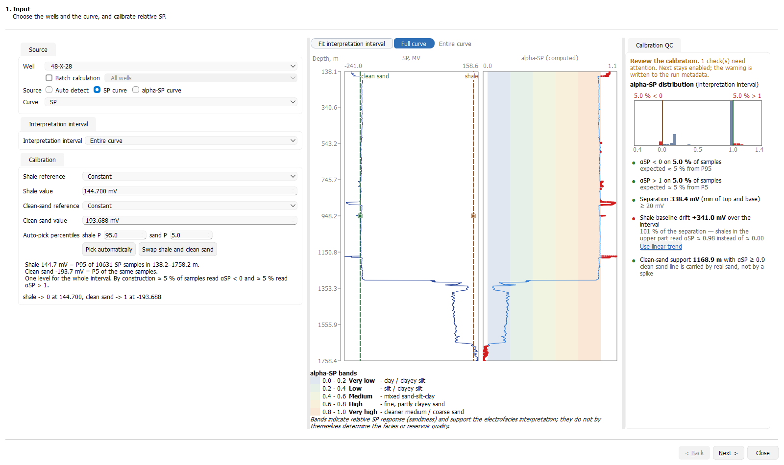
To interpret several wells, select Batch calculation, choose the well scope, and review the Wells list. Its name, source, and selected-zone filters determine which wells run. Selecting both Has SP and Has alpha-SP keeps wells with either curve. The list shows wells that will be skipped and why; source curves, intervals, and calibration are resolved for each well.

2. Context

Context is optional. You can leave Depositional setting, Energy, and Dominant lithology at Unknown. A specific depositional setting narrows the pattern groups compared; Mixed compares all active facies, just like Unknown. Energy and lithology contribute to scoring within those groups without filtering them. If the library contains no facies with the selected lithology, that lithology contributes a neutral score, just like Unknown; the page explains this beside the context fields.

Click a pattern-library card to inspect the group's facies records and distinguishing notes below the cards. Greyed groups are outside the current compared set but can still be opened for inspection; opening a card does not include that group in the identification.

3. Identification

Choose Segmentation: Existing intervals - Zones, Existing intervals - Formations, or Automatic - from the alpha-SP curve. Automatic segmentation derives boundaries inside the interval chosen on Input and does not bridge nulls or gaps. Choose the Pattern library and a Decision rules preset: Conservative, Balanced (the default), or Permissive. Open Expert to adjust the ambiguity threshold, minimum match score, minimum interval thickness, or DTW band width. The preset cards forecast the outcome for the displayed well. Editing Expert values selects Custom when they no longer match a preset; entering a preset's values selects that preset again.

4. Results

By default, the depth tracks fit the selected interpretation interval: Custom interval uses Top and Bottom, Markers range uses the selected markers, and Zones spans all selected zones, including gaps between them. Entire curve shows the full source-curve depth range. Use Full curve to see the surrounding depths, or Fit interpretation interval to return to the selected range. These controls share the same setting on Input, Identification, and Results. On Results, fitting keeps both the alpha-SP and electrofacies tracks aligned and expands to include result boundaries edited beyond the selected range. Clicking a result block selects its corresponding table row and updates the candidate comparison.

Select an interval in the Intervals table or on the track. Confidence shows its match score from 0–1, or the score of the accepted candidate after a manual choice. A library assignment without a scored candidate reads set by hand; a skipped interval has no confidence value. Margin is the score gap to the best rival and is blank when there is no rival. A small margin means the alternatives are close. The selected interval's status reason explains an ambiguous, unclassified, or skipped result, such as a close alternative, a score below the minimum, or unusable samples. Open Messages to review run warnings and skipped-interval notes; batch notes appear with the corresponding well in the run summary.

Review the ranked Candidate facies. Tick A and B beside two candidates to compare them in Observed vs candidates A and B, the observed/A/B descriptor table, and the supporting evidence. The evidence explains the shape and interval descriptors behind each candidate. Use the status filters or Next to review (N) to find intervals that need attention; an ambiguous or weak match should be checked before it is accepted. Hatched Ambiguous blocks show the leading candidate's colour and a question mark, not a confirmed facies.

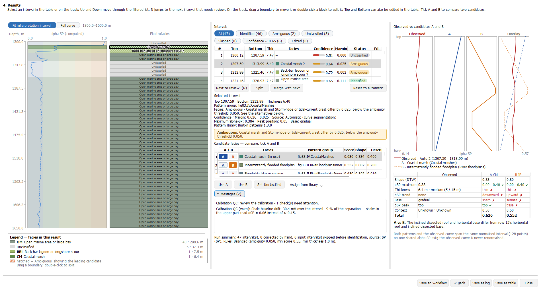
Drag a shared boundary on the result track, or edit Top or Bottom in the table. Moving a shared boundary updates and rescores both neighbouring intervals; intervals separated by a gap keep independent edges. Changed rows briefly flash amber. The Ed. column shows B for a boundary edit, F for a facies edit, and B+F for both. Double-click an interval on the result track to split it at the clicked depth. Split cuts an interval at its midpoint, and Merge with next joins adjacent intervals. Click Use A or Use B to assign a compared candidate, choose another with Assign from library, or click Set Unclassified. A manually chosen facies remains selected after a boundary rescore. Reset to automatic restores the original proposal for the selected interval.

Save as log

On Results, click Save as log. The Facies curve is always included; choose the optional Confidence, Status, and Alpha-SP curves. Edit the output names, then click Save. The default names are ELECTROFACIES, ELECTROFACIES_CONF, ELECTROFACIES_STATUS, and ASP_EF respectively. Confidence, Status, and Alpha-SP are selected by default when available. The wizard remembers your output choices between sessions. Alpha-SP is offered only when this run calculated it from SP, and is saved only for those wells, not for wells using an existing alpha-SP input. In a batch, the same curve names are used on every interpreted well. Selected curve names must be nonempty and distinct.

The facies curve stores fixed Pattern Library facies codes, with 9001 for Ambiguous and 9002 for Unclassified. Confidence values range from 0–1. Status codes are 1 Identified, 2 Ambiguous, 3 Unclassified, 4 Skipped, and 5 Manual. The facies curve uses the Lithology display style in well-log views and can be shown as categorical data in Well correlation.

Save as table

On Results, click Save as table to save the reviewed interpretation, including manual edits. Edit Table name (default: Electrofacies), then click Save. Each interpreted well gets a table under Statistics / Tables, named <base> - <well>. Each interval row contains Top, Bottom, Thickness, Facies code, Facies name, Confidence, Status, and Manually edited, followed by pattern-match details including score, library, and interpretation origin.

Select Run parameters to also save a parameter table named <base> run - <well> and the parameters as JSON in the interval table description. This option is selected by default; inspect Run parameters preview before saving. In a batch, each well records its own parameters.

Logs and tables are saved separately; use both actions if you need both outputs. If an output name already exists, choose Yes to overwrite it, No to keep it and save the new output under a versioned name, or Cancel to save nothing. The confirmation lists the actual saved outputs and their names for each well, plus skipped wells and their reasons. The wizard stays open after saving. For a batch, the Run summary lists each well under Well, Source, Interval, and Result; processed rows name the source curve and interval, while skipped rows give the reason.

Save to workflow

Save to workflow opens Workflow task outputs. Select Save as log, Save as table, or both, choose the optional outputs and edit their names, then click Save. This stores the current setup in the Workflow without writing a facies result. Reopening the saved workflow restores its setup, including the well scope, source, interval, calibration, context, identification settings, output choices, and output names. The task writes those selected outputs under those names when it runs; Alpha-SP is written only for wells where it is calculated from SP. A reopened task offers Save to update its settings. Use Close to leave the wizard.