Time table calculation for tomo update
Travel time calculation for depth migration process (PSDM stage)
Theory
Time table calculation module generates an input data file for depth migration module (Kirchhoff PreSDM - file in/out - migration TT), this file is depth migrated common image gathers that are used as well for tomography updates. The time table calculation module is an essential component of the PSDM (Prestack Depth Migration) workflow and is required for every execution of the depth migration process.
In the Prestack Depth Migration (PSDM) stage, travel time calculation is essential for accurately mapping seismic data to depth. The process begins with solving the eikonal equation, a fundamental mathematical model that describes wavefront propagation:
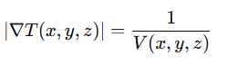
Here, T(x,y,z) is the travel time at each point in the subsurface, and V(x,y,z) is the velocity model. This equation ensures that travel times account for variations in velocity, which is crucial for imaging complex subsurface structures.
Next, ray tracing techniques are applied to model the paths that seismic waves take as they travel through the earth. Starting from a source point, rays are traced along the direction of the travel time gradient (∇T) using Snell's law and the velocity field. For each ray path, the total travel time is calculated by integrating along the ray trajectory:
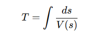
where ds is the incremental distance along the ray. This integration ensures that travel time incorporates the effects of varying velocities along the ray path.
Finally, the computed travel times are used to update the depth image. Each seismic trace is mapped to its corresponding subsurface location based on the calculated travel times. By iteratively refining the velocity model and recalculating travel times, the PSDM process produces high-resolution depth images that accurately represent the geological structures. This iterative workflow ensures that errors in the initial velocity model are progressively corrected.
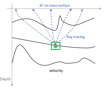
 Source & Receivers are having a constant datum value and Bin (CMP) elevations are the actual values and lesser than the datum value. We have to annotate the Source_Elev, Source_Datum, Receiver_Elev, Receiver_Datum, Bin_Elev, Inline (In case of 2D it shall be zero) and Crossline to confirm that all the required headers are present and correct.
Time table calculation for tomo update requires rectangular shape of XY-area for the input velocity data, therefore you should use module: Merge velocity gathers. It can create a rectangular XY shape of the velocity. Otherwise Time table calculation for tomo update will show an error message about irregular XY shape area of the velocity!
Input data
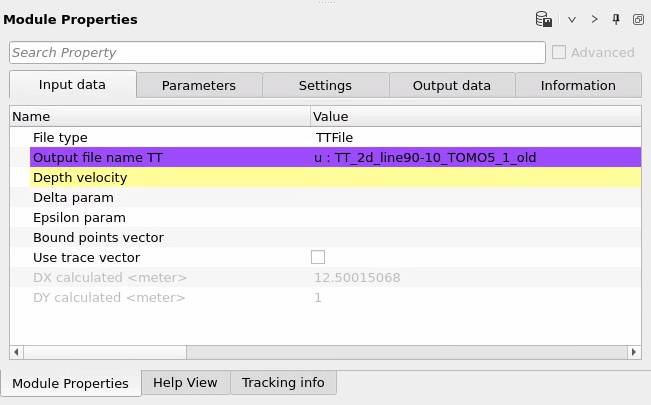
File type
:
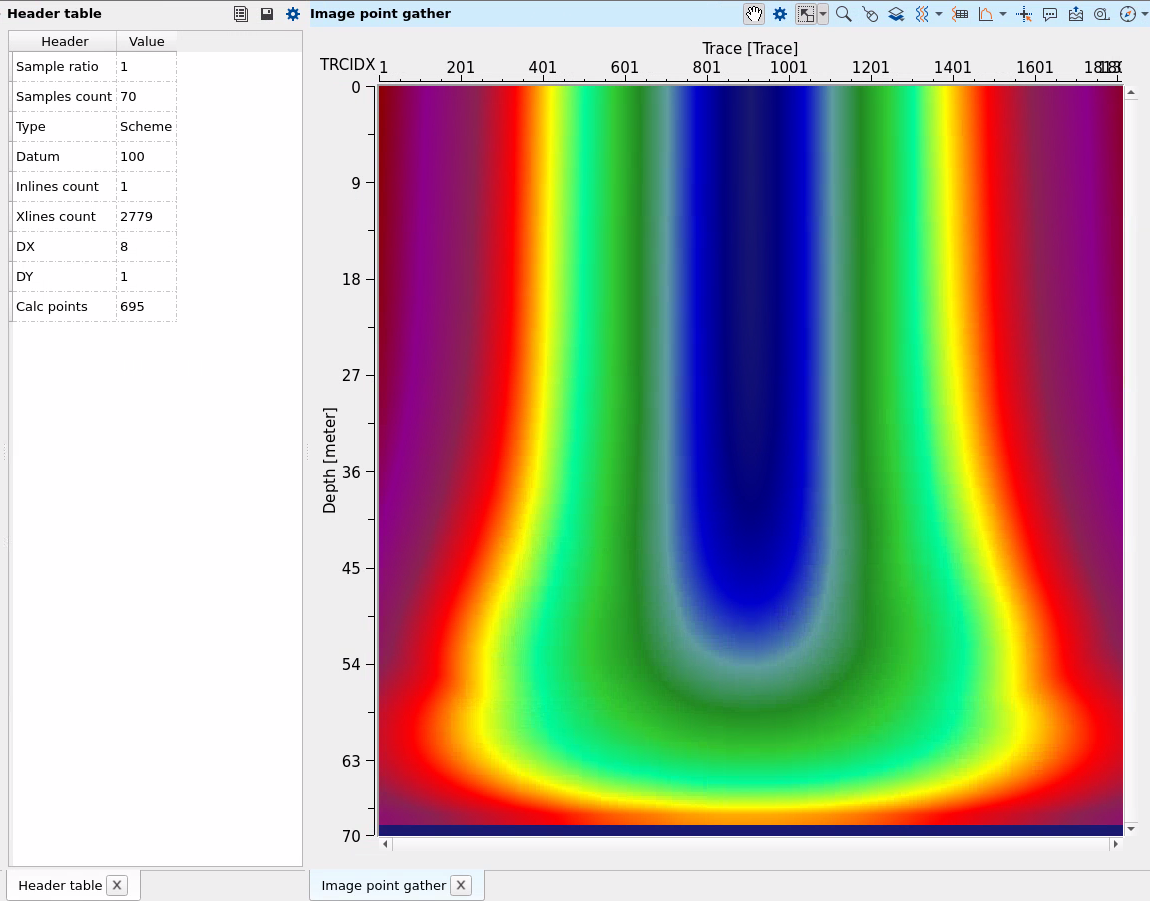
TTFile - output file will be in the internal data base (g-Platform) and format is Time table (TT). TT file can be viewed in TT viewer module for QC purposes (see example in the example part of this documentation).
GSD - output file will be in the internal data base (g-Platform) and format is Geomage Seismic Data (GSD).
TTFile and GSD - output files will be in the internal data base (g-Platform) and formats are: Geomage Seismic Data (GSD) and Time table (TT).
Output file name
define an output seismic TT file name in case of using GSD option.
Output file name TT
define an output TT file names in case of using TTFile option.
Depth velocity
connect to the input velocity model.
Delta param
connect to the input Delta Thomsen model (optional).
Epsilon param
connect to the input Epsilon Thomsen model (optional).
SGY handler V
connect seismic data handler to the input velocity model (optional).
Trace headers V
connect headers to the input velocity model (optional).
SGY hander D
connect seismic data handler to the input delta model (optional).
Trace header D
connect headers to the input delta model (optional).
SGY hander E
connect seismic data handler to the input epsilon model (optional).
Trace header E
connect headers to the input epsilon model (optional).
Bound points vector
connect to the input polygon for limit calculation area (you should prepare polygon item via Polygon picking module). Area that is out of the polygin will be not calculated (optional).
Use trace vector
enable this option in case you don't have enough RAM on the local machine to upload all input attributes (Velocity, Delta, Epsilon), so there are 6 input parameter will be activated (SGY handler V, Trace headers V, SGY handler D, Trace headers D, SGY handler E, Trace headers E). Please, pay attention that you have to enable as well other parameter called Use boundaries in the paramter's tab.
DX calculated
step for calculation along X direction (optional).
DY calculated
step for calculation along Y direction (optional).
Parameters
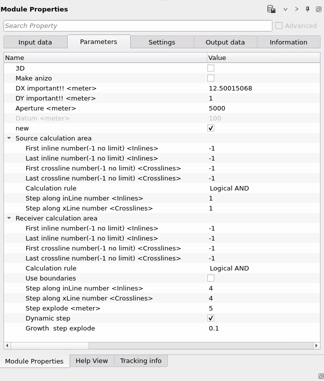
3D
enable this option in case of 3D seismic data.
Make anizo
enable this option in case of using Thomsen parameters Delta and Epsilon.
DX important!!
bin size X distance (CMP interval) in meters, it is better to define it manually in accordance with read value from the seismic data (without big number of decimal places, for example 12.5 is good, 12.49002345 is bad). Also, this value is updated automatically when you connect input velocity in the Input data tab (be careful if you would like set distance manually!).
DY important!!
bin size Y distance (CMP interval) in meters, it is better to define it manually in accordance with read value from the seismic data (without big number of decimal places, for example 12.5 is good, 12.49002345 is bad). Also, this value is updated automatically when you connect input velocity in the Input data tab (be careful if you would like set distance manually!).
Aperture - you need to set the calculation aperture for the time table to be larger than the migration aperture by max offset / 2. For example, if you plan to run migration with an aperture of 3000 m, the time table aperture should be set to at least 4500 m. Regarding running calculations on the server: If the time table calculation was not completed for any reason, you can restart it, and the process will resume from the point where it stopped previously (i.e. restart the module execution in the g-Navigator).
Datum - datum plane in meters. Automatically takes from trace headers datums of the input velocity (RECEIVER_DATUM, SOURCE_DATUM). Note that the datum plane for depth velocity model will be set above the maximum elevation of the topography. This means that ray tracing will begin from this constant (horizontal) line, then pass through the topography, and continue further.
Source calculation area - parameters for area calculation, limitation, decimation, polygon usage. These parameters significantly affect the calculation time as well as the quality (detail) of the solution. For example, setting the parameters to 4x4 & 4x4 will result in longer computation times but provide better detail. On the other hand, if you use 10x10 & 10x10, the seismic image may show “upward bending” of reflections, indicating a loss in velocity accuracy due to interpolation. Therefore, it is crucial to conduct tests to determine the optimal travel-time calculation step.
ray initialization starts from receivers and goes to the sources positions on the topo-surface (from bot to the top), therefore we can do increment for receiver calculation area (receiver step. line receiver step), and try to avid to make big decimation for sources (in ideal situation set it to 1, especially for 2D data). You should do accurate tests for these parameters, check if there is loss of quality in the resulting CIG data (after depth migration).
In the parameters, you can specify a polygon to trim the edges, ensuring that time is not wasted on calculating empty cells.
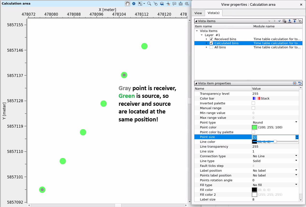
It is also very important to check the positioning map of RCV (receivers) and SP (sources). The points must align so that each RCV includes an SP. This alignment ensures proper near-offset calculations; otherwise, issues will arise. The number of SP points can exceed RCV points, as in cases where RCV is set to 15x15 and SP to 5x5, but it is critical that every RCV contains an SP:
To generate a stack quickly, calculate travel times (TT) only along the line of interest. This approach should be fast enough without requiring TT calculations with, for example, a 3 km aperture on either side of the line.
For instance, if in the project, the spacing between RCVs was set to 15x15 (equivalent to 300x300 meters) and SPs to 5x5 (100x100 meters). Considering that an updated time table calculation module was used (Time Table Calculation for Tomo Update), where source initiation occurs inversely from receivers, SP points could be configured with a denser spacing of 5x5.
First inline number(-1 no limit)
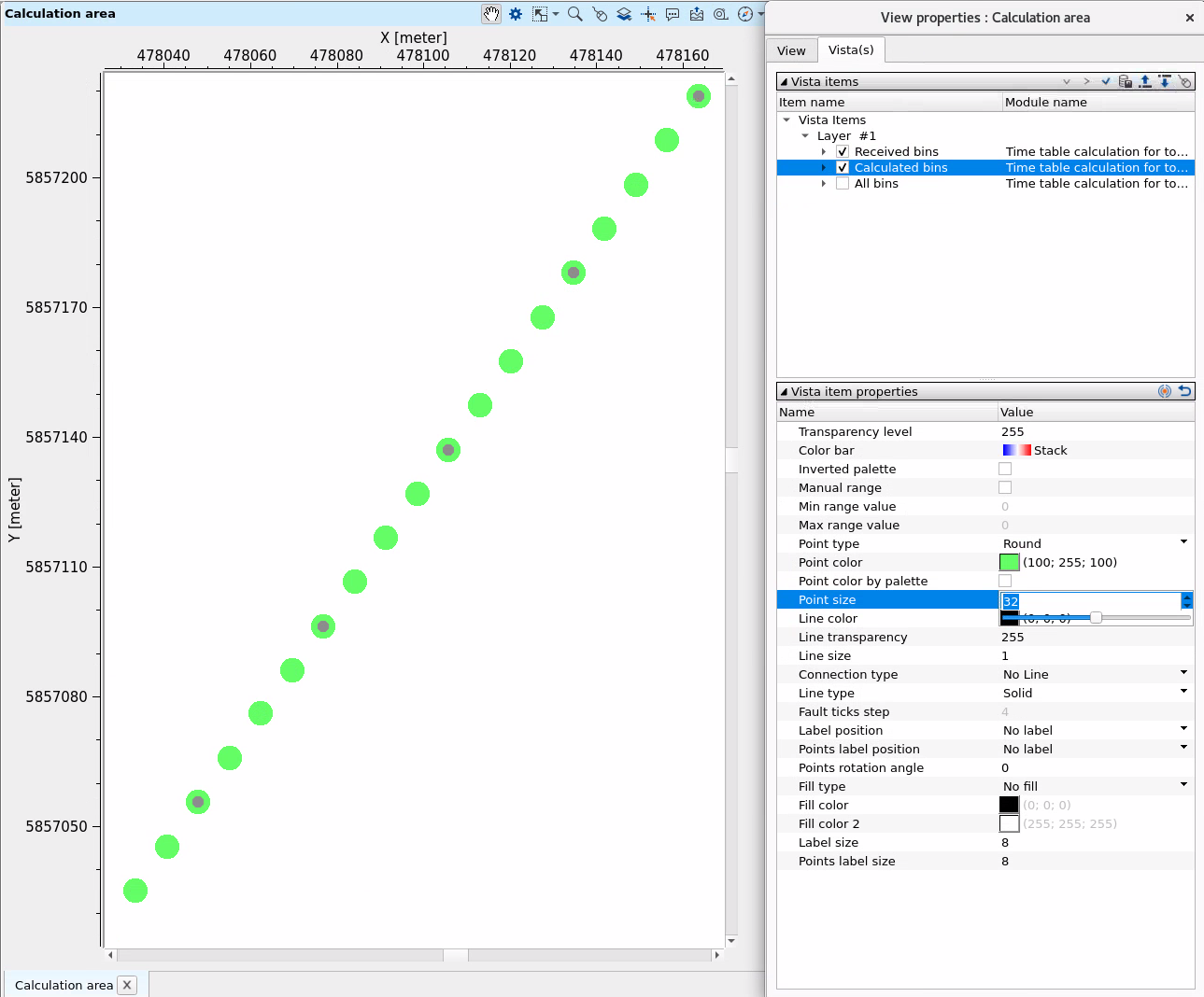
first source line number of the points for ray path initializations. Starts from 1. Use Visual vista item for QC:
Last inline number(-1 no limit)
first source line number of the points for ray path initializations. Starts from 1. Use Visual vista item for QC.
First crossline number(-1 no limit)
first source xline number of the points for ray path initializations. Starts from 1. Use Visual vista item for QC.
Last crossline number(-1 no limit)
last source xline number of the points for ray path initializations. Starts from 1. Use Visual vista item for QC.
Calculation rule { Logical AND, Logical OR }
parameter for changing a logic of source and receiver point creation (regular math expression).
Step along inLine number
decimation step in inline numbers along source inline direction.
Step along xLine number
decimation step in xline numbers along source inline direction.
Receiver calculation area
the same as source calculation area, but the meaning is different in terms of receiver positions are actually points of ray initialization (but source is final position of ray arrival).
First inline number(-1 no limit)
first receiver line number of the points for ray path initializations. Starts from 1. Use Visual vista item for QC.
Last inline number(-1 no limit)
last receiver line number of the points for ray path initializations. Starts from 1. Use Visual vista item for QC.
First crossline number(-1 no limit)
first receiver xline number of the points for ray path initializations. Starts from 1. Use Visual vista item for QC.
Last crossline number(-1 no limit)
last receiver xline number of the points for ray path initializations. Starts from 1. Use Visual vista item for QC.
Calculation rule { Logical AND, Logical OR }
parameter for changing a logic of source and receiver point creation (regular math expression).
Use boundaries
enable this parameter in case of using polygon for limitation area calculation. Pay attention you need to connect input polygon to Bound points vector parameters which is located in the Input parameters tab.
Step along inLine number
decimation step in inline numbers along receivers inline direction.
Step along xLine number
decimation step in inline numbers along receivers xinline direction.
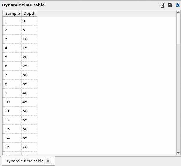
Step explode - vertical step in meters for ray initialization. Additionally, you can use the next two parameters to make this step dynamic (i.e. not a constant step, but increase in accordance with depth).
Dynamic step - parameter for making Step explode dynamic (i.e. not a constant step, but increase in accordance with depth). Use QC Visual Vista Item to see step intervals for rays initializations:
Growth step explode
use this coefficient to change Dynamic step (increase or decrease).
Cut V - the calculation will be faster as unnecessary velocity data is excluded during processing. For example, the calculation progresses step-by-step based on the discretization step specified in the parameters, such as 100 meters: first 100, then 200, then 300, and so on. Each time, the module removes velocities below the current explosion level to avoid unnecessary computations.
Settings
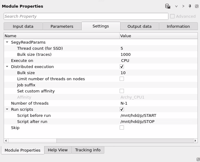
SegyReadParams
parameters for setting advanced parameters of reading seismic traces from disk:
Thread count (for SSD)
amount of treads for reading seismic traces from disk.
Bulk size (traces)
size of a chunk (data portion) for reading seismic traces from disk.
Execute on { CPU, GPU }
- select which type of processor will be used for calculations: CPU or GPU.
Distributed execution
if enabled: calculation is on coalition server (distribution mode/parallel calculations).
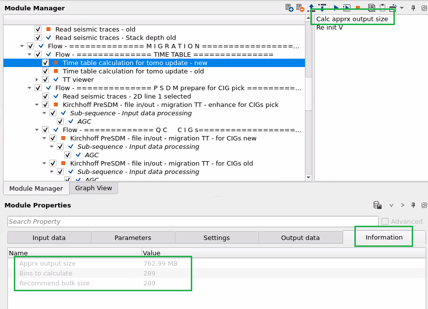
Bulk size
chunk size is RAM in megabytes that is required for each machine on the server (find this information in the Information, also need to click on action menu button for getting this statistics):
Limit number of threads on nodes
limit numbers of of threads on nodes for performing calculations.
Job suffix
add an job suffix.
Set custom affinity
an axillary option to set user defined affinity if necessary.
Affinity
add your affinity to recognize you workflow in the server QC interface.
Number of threads
limit number of threads on main machine.
Run scripts
it is possible to use user's scripts for execution any additional commands before and after workflow execution:
Script before run
path to ssh file and its name that will be executed before workflow calculation. For example, it can be a script that switch on adn switch off remote server nodes (on Cloud).
Script after run
path to ssh file and its name that will be executed before workflow calculation.
Skip - switch-off this module (do not use in the workflow).
Output data
Output geometry
output geometry item for QC.
Dynamic time table
output dynamic time table item for QC.
Information
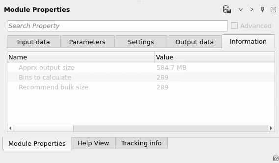
Apprx output size
approximate size o the output Time Table file on the disk.
Bins to calculate
how many bins will be calculated (use it for distribution settings on coalition server: number of bins per node).
Recommend bulk size
recommended bulk size for distribution settings on coalition server per node.
Actions
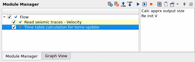
Calc apprx output size
calculate approximate size of the output TT file (on disk). Resulting information you can find in the Information tab:
Re init V
update initialization input velocity in case of reconnection.
Examples
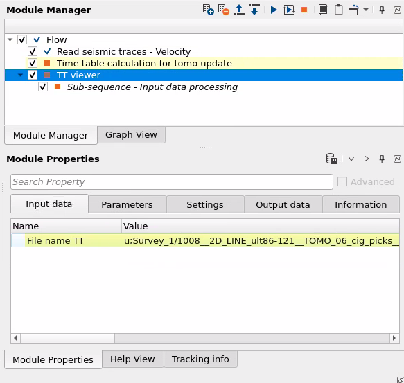
Workflow example and Time table calculation for tomo update parameters:
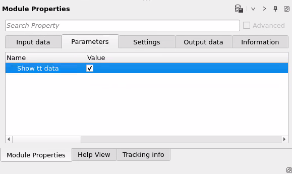
Time travel can be visualized via TT viewer module:
Related articles
 If you have any questions, please send an e-mail to: support@geomage.com
References
Vidale, J. E., 1988, Finite-difference calculation of travel times: Bulletin of the Seismological Society of America, 78, 2062-2076.